
Data and modelling are very important components of asset management. Roads, bridges and other transportation assets do not last forever. They have a limited service life which is affected by traffic loading and environmental impacts such as heating and cooling and changes to moisture content, etc.
In order to effectively manage transportation assets, it is necessary to have a complete inventory of the assets to be modelled. Once the inventory is established, the condition of the asset should be determined. This may include variety of distresses, depending on the asset type.
Once sufficient condition information is collected, this data can then be used to modelling the performance of the asset so that its future condition can be predicted. This will then allow planning and budgeting for future maintenance and rehabilitation treatments to cost-effectively manage the asset.
Investment decisions for assets may also be allocated based on risk. For example, funding may be allocated to assets required to access remote communities. If the asset is compromised, residents may not be able to obtain access to essential services.
Asset management systems typically include tools for the full life-cycle evaluation of an agency’s assets. Lifecycle plans may be used to demonstrate how funding and/or performance requirements are achieved through appropriate maintenance strategies with the objective of minimizing expenditure while providing the required performance over a specified period of time.
A key aspect of the development of asset management is data collection. The way in which road organizations collect, store, and analyze data has evolved along with advances in technology, such as mobile computing (e.g., handheld computers, laptops, tablet notebooks, etc.), sensing (e.g., laser and digital cameras), and spatial technologies (e.g., global positioning systems (GPS), geographic information systems (GIS), and spatially enabled management systems).
Bridges are normally only second to pavements in magnitude of network expenditures. Bridges also significantly affect the safety and performance of a roadway network. Bridge condition inadequacies can affect the traveling public as well as an agency. Bridges that deteriorate into poor condition often require more frequent maintenance and on demand repairs that cause traffic disruptions and place administrative and economic burdens on the agency. Bridge performance is also impacted by load capacity and geometric inadequacies that may cause restrictions on truck sizes and allowable weights, or may cause waterways to overtop the bridge at unacceptable frequency for the roadway classification. These factors can also affect roadway network performance as bridge inadequacies may cause traffic to take alternate routes.
Data collection is also valuable for other roadway features or asset classes when they affect safety, performance, or cost to manage the roadway network. Tunnels, slopes, retaining walls, sign structures, drainage structures, guide rails, etc. are included in this category.
The use of these systems and technologies has enhanced the data collection and integration procedures necessary to support the analyses and evaluation processes needed for asset management but at the same time has led organizations to collect very large amounts of data and create vast databases that have not always been useful or necessary for supporting decision making processes.
Asset condition data collection activities should be designed to support asset management decision processes at different levels. This should include a rational evaluation of what data should be collected to cost-effectively support the asset management decision. As asset management includes a variety and type of assets, one type of data, for example traffic, may be needed for multiple applications. Information for all asset needs should be considered when establishing the data collection program. Once the data needs are established, a data collection plan can be developed to outline the type and frequency of data collection. The plan should include procedures for quality control validation of the data. Once the data quality is confirmed, it can then be transformed into performance indices.
One of the key components of the management of assets is to inventory and document that assets that are the responsibility of an organization along with their current condition (OECD 2001). Different types of data are required for the effective management of the road infrastructure (PIARC 2004). This may include inventory information, age, remaining life and performance information (e.g. pavement smoothness, bridge structural capacity, etc.). Data collection technologies and data needs vary depending on which infrastructure element is evaluated (Birmingham 2002) and on road organization needs and culture as well as the availability of economic and human resource. Therefore, there is no one-size fits-all approach for asset management data collection.
The data collected should support the following objectives:
In today’s big data world it is possible to gather data on just about anything, but the primary objective should be to collect only data that will measure progress toward the defined goals and help road organization to make decisions.
The data needed by any road organization are those that influence (World Bank 1997):
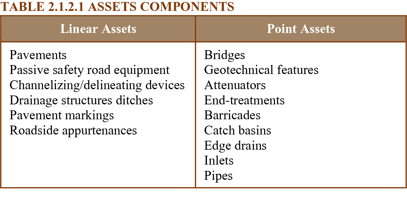
In principle, asset management data falls into three main types and can be grouped as follows:
Inventory and condition data refer to the key infrastructure areas or the primary asset components including liner and points assets, as shown in table 2.1.2.1.
Regardless of the maturity level of a specific road organization, it is imperative that a data management strategy be defined (Telli 2010). A data management strategy may comprise the following:
The following questions should be considered when deciding what data to collect:
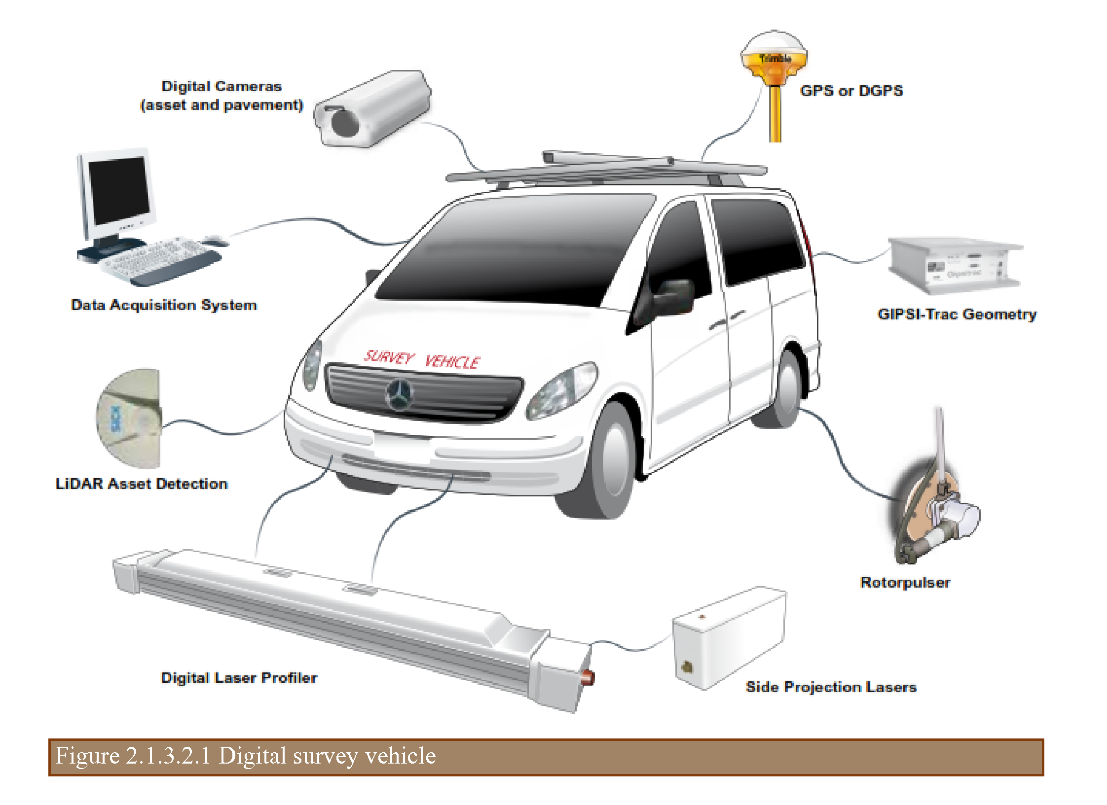
The data collection process begins with the establishment of data needs. Data needs will vary from agency to agency depending on the complexity of the transportation network, the level of maturity of the agency, available technology and indices used to reflect the condition of the assets (U.K. Roads 2013). For relatively small and less complex networks, this may consist of a visual survey to establish an overall condition index. Larger networks in more developed countries my include the use of digital survey vehicles and other equipment that measure asset attributes using digital imaging, laser technology and equipment that measures the in-situ strength of the asset. Regardless of the method used, quality control and assurance procedures should be established to ensure the consistency of the condition assessments. While multiple asset attributes may be measured to assist in making detailed project level maintenance and rehabilitation decisions, these attributes may be combined to provide a single measure of asset condition for network level asset management.
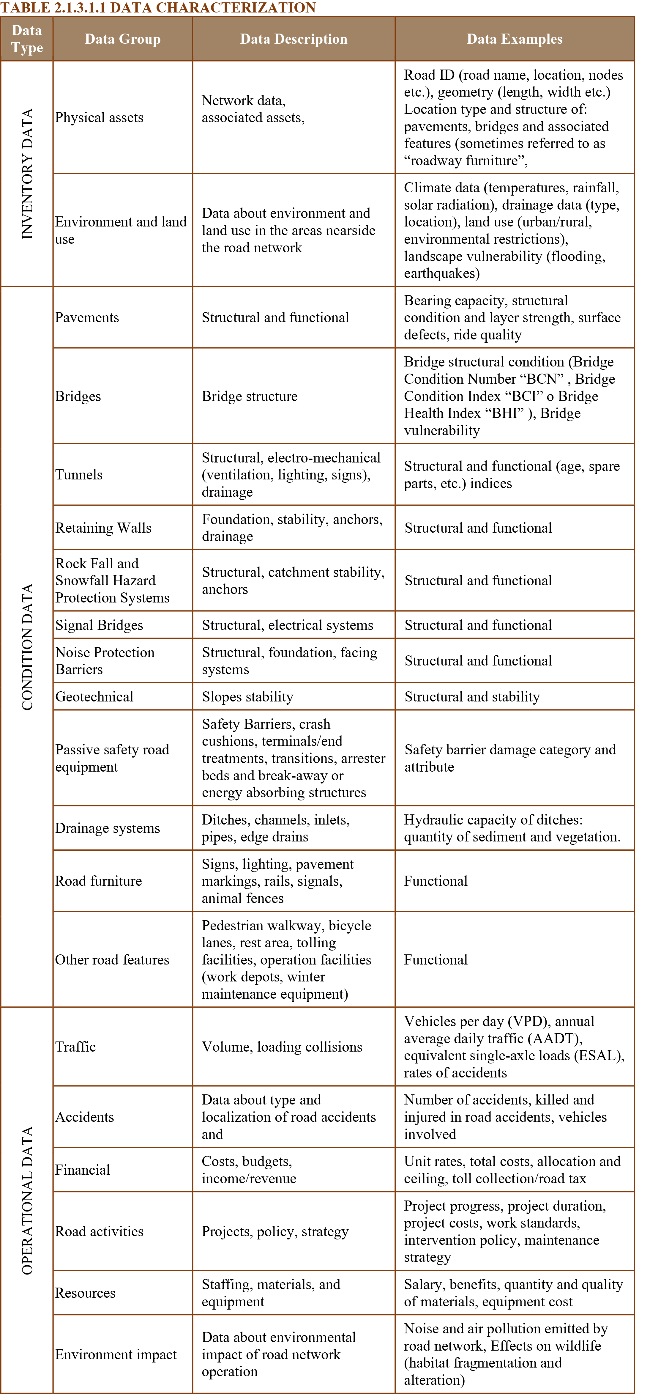
Road data can broadly be categorized into various data groups, as shown in Table 2.1.3.1.1.
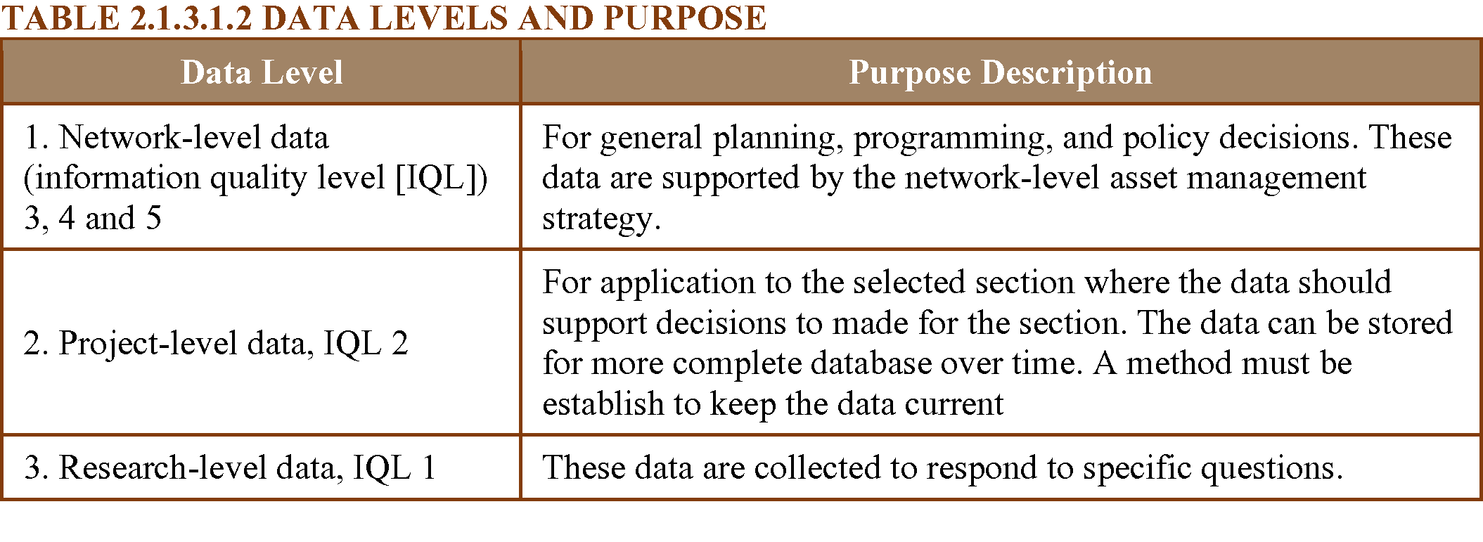
When collecting data, the road organization needs to consider the level of analysis for which it will be used, as summarized in Table 2.1.3.1.2.
The amount of data to be collected and the frequency at which data will be collected will depend on the following:
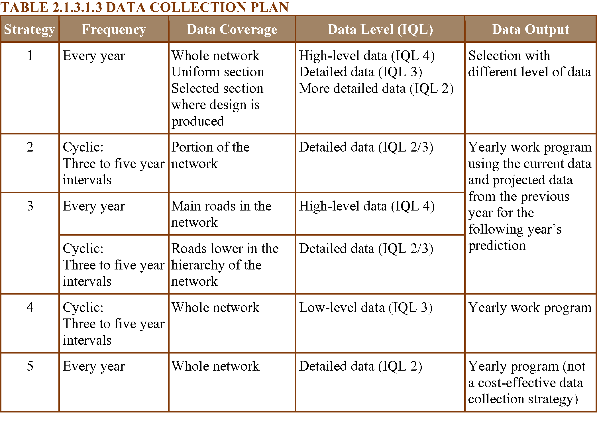
The road data collected should be programmed or strategized to match their function in the asset management process and the data IQL. A data collection program that can be adapted by other transportation agencies is shown in Table 2.1.3.1.3.
Traditional methods used for the collection of Asset Management data include manual, automated, semi-automated, and remote collection. For manual collection the data are documented either with pen and paper, or in more recent cases, with handheld computers equipped with GPS. Automated collection involves the use of road sensors or multipurpose vehicle equipped with a position/navigation system (e.g. distance-measuring device and GPS antennas), a combinations of different sensing technologies (e.g. video cameras, gyroscopes, laser sensors, etc.) as well as computer hardware in order to capture, store, and process the collected data. Semi-automated methods involve similar equipment as the completely automated method but with a lesser degree of automation. Remote Collection method pertains to the use of satellite imagery and remote sensing applications (e.g. high-resolution images acquired through satellites, aerial photos, etc.).
In the last decades, data collection have shown a trend toward automation, computerization and digitalization. Furthermore, there is a great expectation of taking the advantage of big data (e.g. data collected by users by smartphone) in the asset management process.
The following factors determine the selection of technologies and equipment for data collection:
It will be advantageous if the equipment or methods employed in data collection can collect road data in a single operation so that the collection will be cost-effective and consistent in referencing. The equipment for data collection can be divided into two main categories:
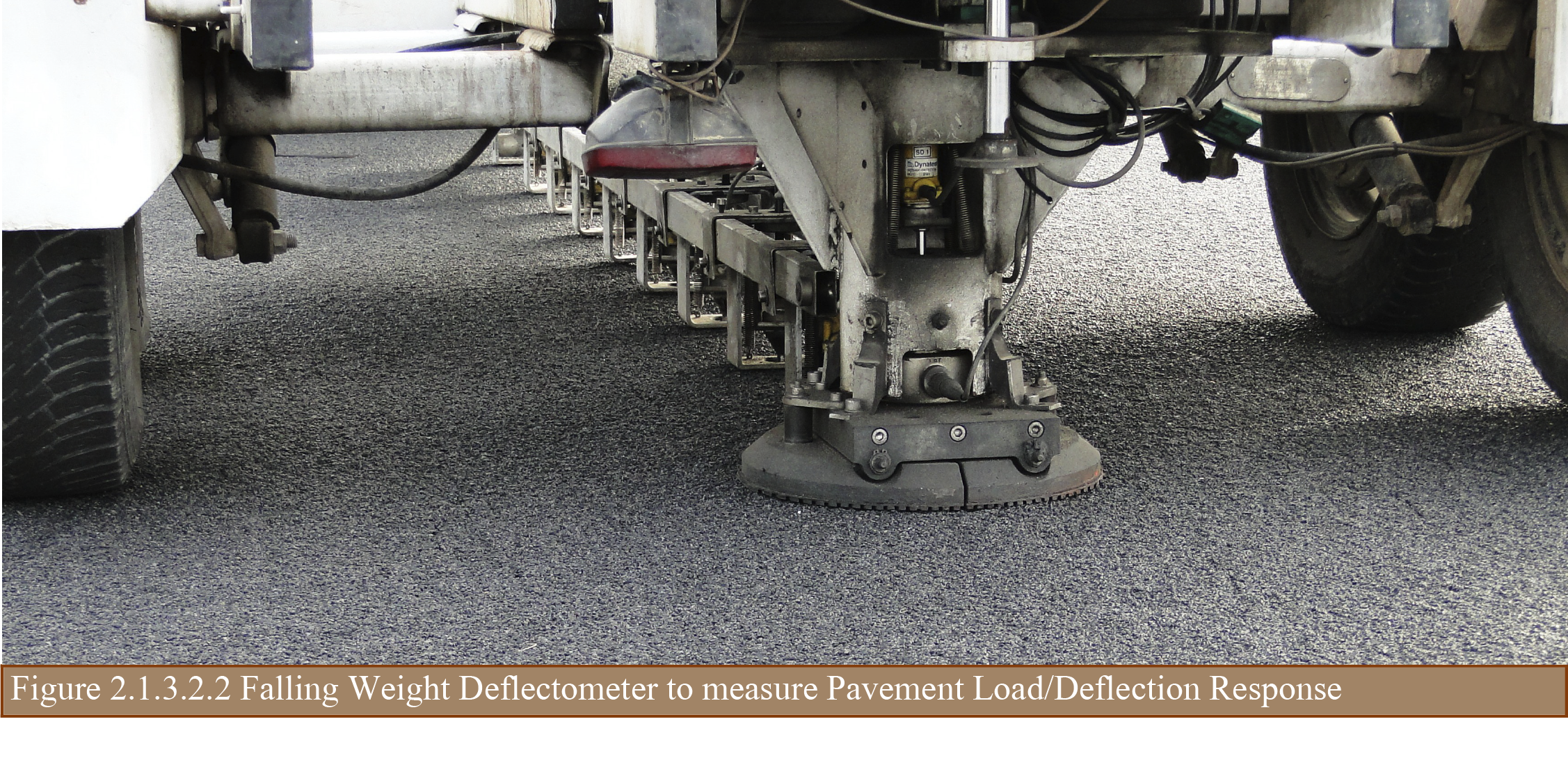
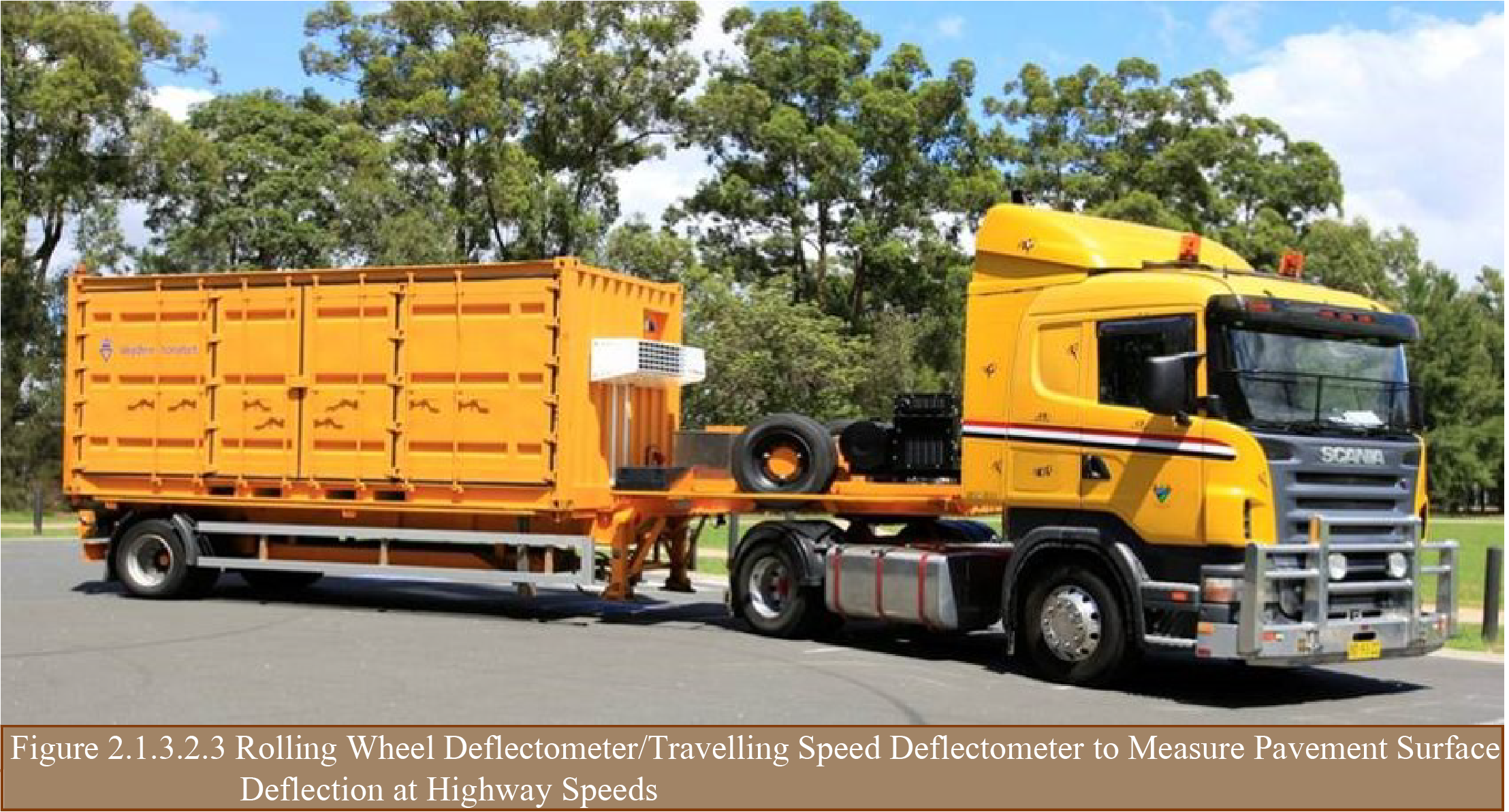
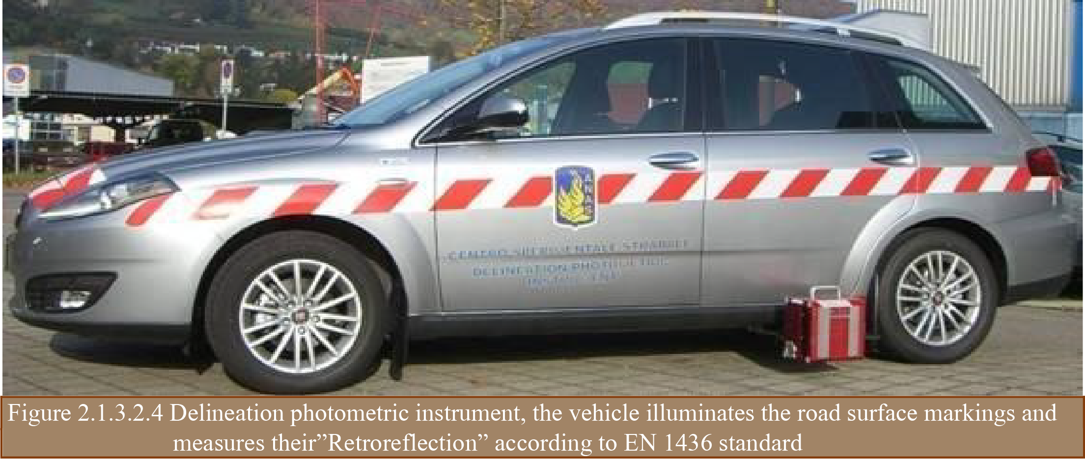
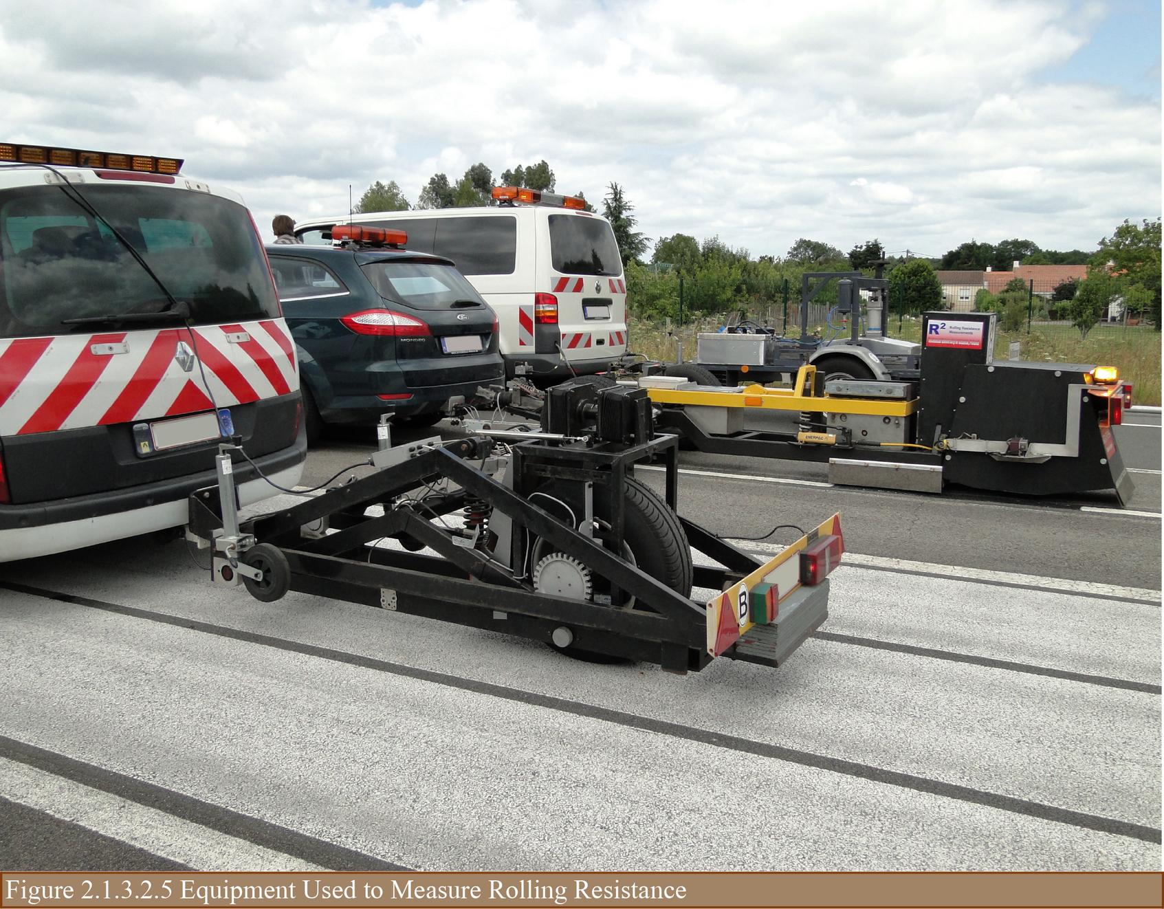
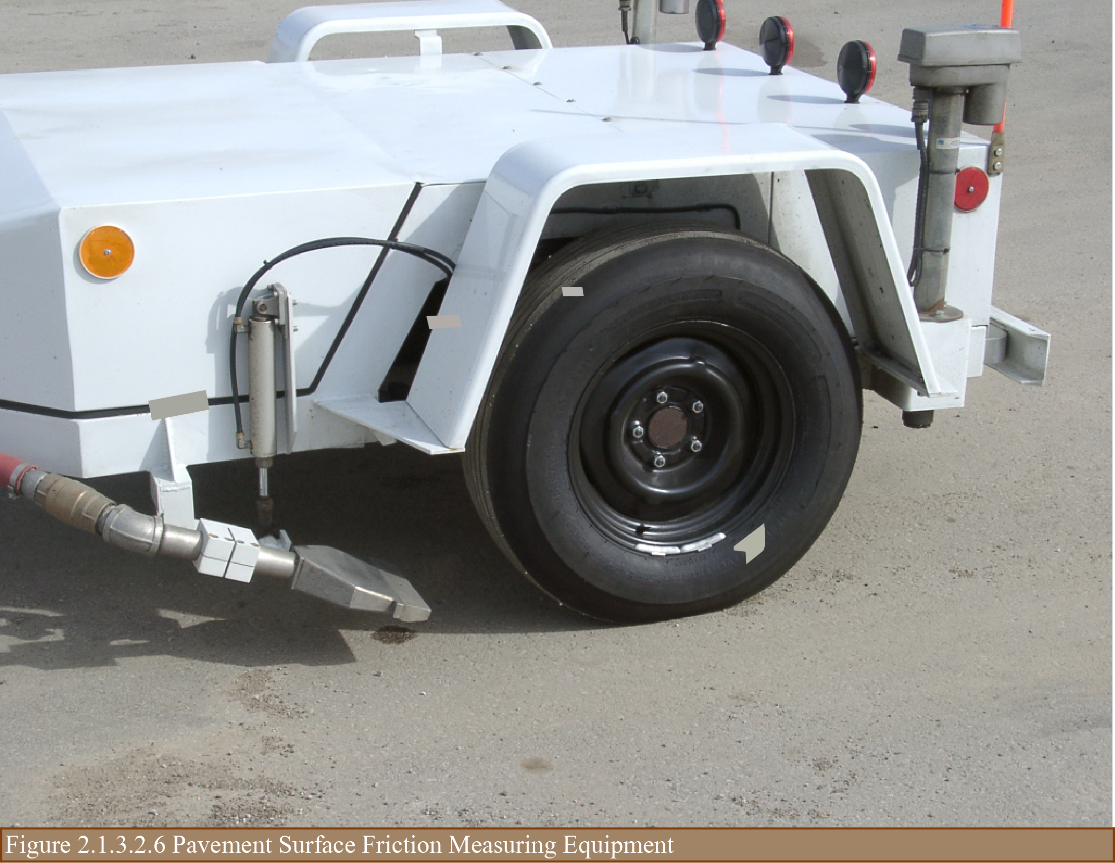
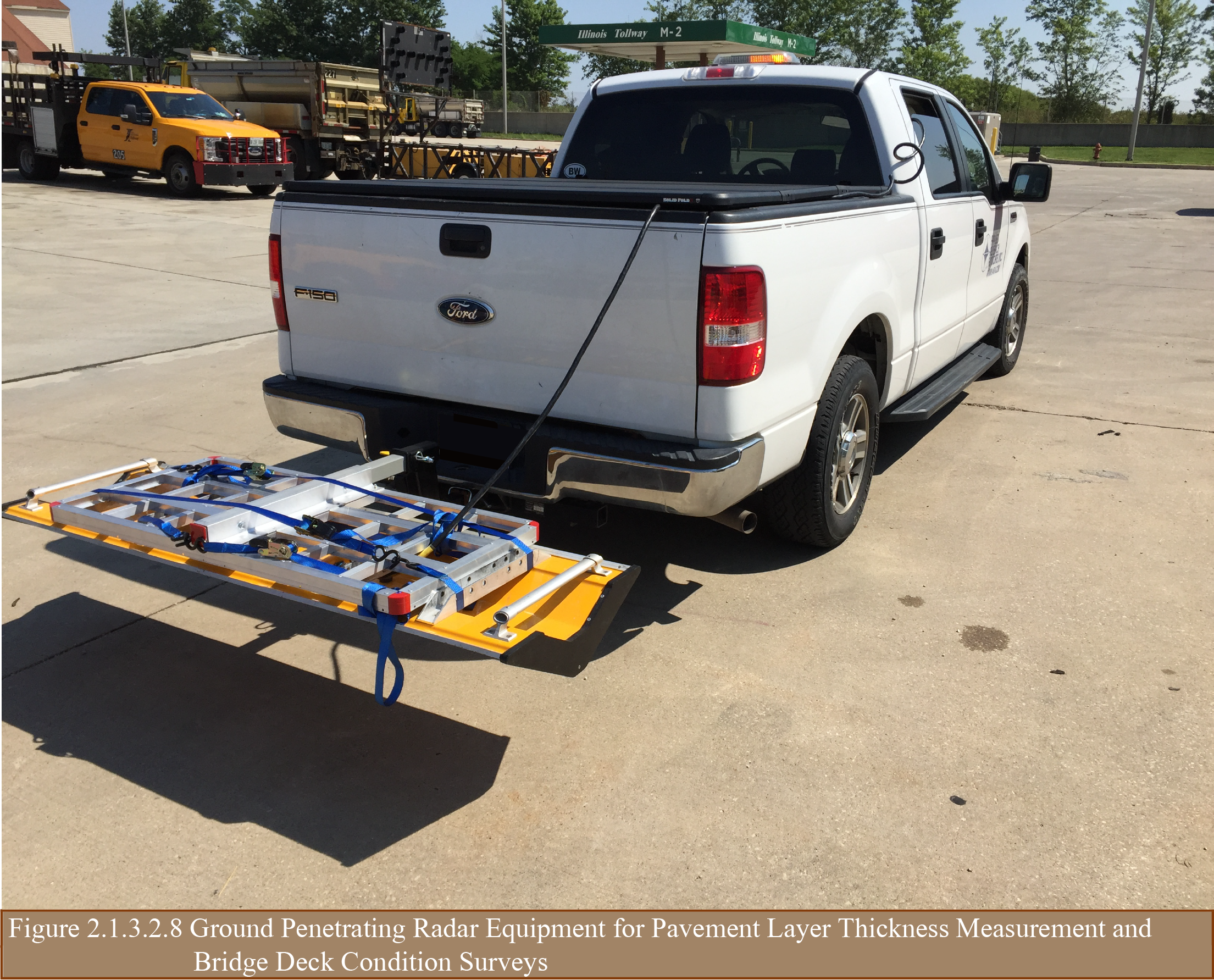
Various other types of technology for data collection are widely available, e.g., drones to inspect bridges, surface profilers, Falling Weight Deflectometers (FWD) for measuring the structural capacity of the pavement and to back-calculate pavement and subgrade layer properties, or continuous deflection measurement systems such as the Rolling Wheel Deflectometer (RWD), RWDVision and Travelling Speed Deflectometer (TSD), equipment to measure paint marking condition and retroreflectivity, rolling resistance, pavement surface friction, light detection and ranging (LiDAR) to map roadside equipment and features, ground penetrating radar (GPR) to determine pavement layer thicknesses and bridge surface condition and rolling resistance equipment. PIARC has recently completed a special report (PIARC 2018) on the use of unmanned aerial systems use for asset condition inspection and data collection.
Figures 2.1.3.2.1 through 2.1.3.2.9 show some examples of data collection equipment and systems.

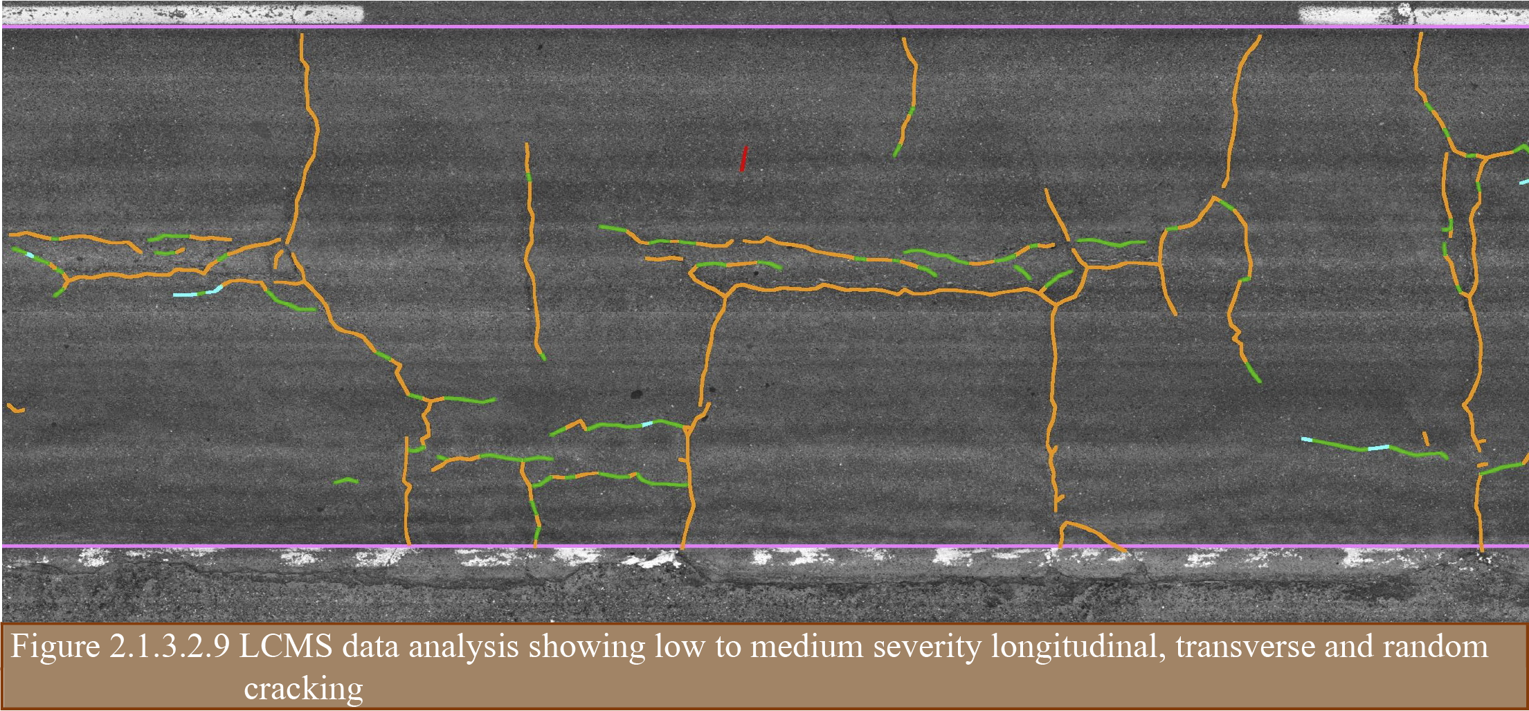
Recent additions to digital survey vehicles include the use of laser crack measurement systems (LCMS). The LCMS is a high-speed 3D laser scanning system that scans a pavement width of 4 m using 4,000 points, and provides a transverse accuracy of 1 mm and a vertical accuracy of 0.5 mm. e frequency is operator-configurable between 5,600 or 11,200 Hz. The resulting resolution and accuracy is 5 to 10 times that which is available from typical mobile LiDAR systems.
Additionally, the LCMS is capable of a fully automatic inspection of the pavement condition, and can measure the following key parameters:
An example of the LCMS crack detection output for an asphalt pavement surface is shown in Figure 2.1.3.2.9.
Bridges are different from other asset classes because they have many features, all of which significantly impact safety, performance, and management costs. Therefore, bridge data is often extensive and complex. The data that supports assessment of safety, performance, and cost include bridge condition data and bridge inventory data such as bridge type and material, service and usage, geometry, load capacity, and potential work needs and costs. Bridge inventory and condition data is collected to support management of individual bridges as well as management of the roadway network.
With respect to condition data, there are different systems of inspection and data collection. One system can be termed general condition rating assessment. Following this system, the major components of a bridge are each independently assessed for condition. Major components include the deck, superstructure, and substructure. Each component is assigned a single numeric value representative of the overall condition of the component. An example of a general condition rating numeric scale is shown in Table 2.1.3.1.4.
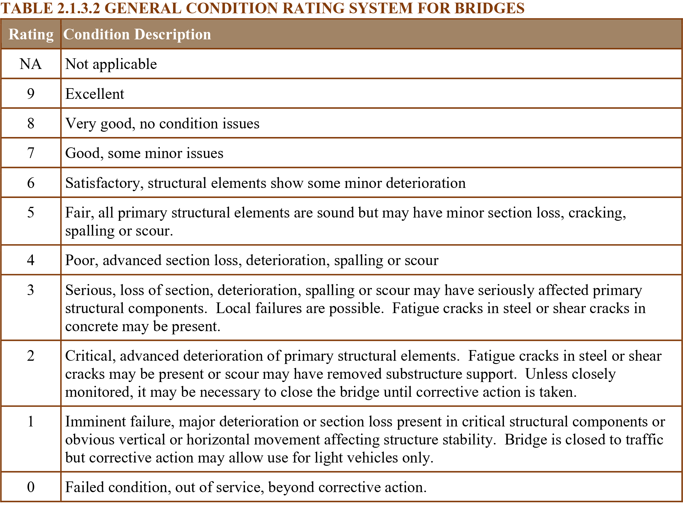
Bridge owners use the general condition ratings to assess the overall condition of bridges and support basic bridge management activities such as identifying high level bridge needs, establishing performance measures, and establishing intervals between inspections.
Another system of condition inspection and data collection is termed element condition assessment. This system subdivides the components into elements that are more granular than components, and it quantifies the type, severity, and extent of defects that are present. First, the unique elements of a bridge for which condition data can be collected are identified. Then the amount of each element is quantified with respect to its size (area or length) or number of elements. During each inspection, the condition of each element is evaluated and the total quantity is distributed among several condition states depending on the type and severity of defects. The use of four condition states is common where condition state number one represents a like-new condition and condition state number four represents a severe condition that warrants structural review, repair, or replacement. This system is also valuable because it identifies the condition of features that are vital to protecting the bridge and preventing deterioration such as protective deck overlays, deck joints, coatings, and erosion protection. The condition of these elements significantly affect bridge service life and life-cycle cost to manage bridges. Bridge owners can use the element condition data for advanced bridge management activities such as accurate identification of bridge maintenance, preservation, and repair needs and associated costs, detailed performance measures that focus on specific bridge features (for example protective systems that extend service life), and asset valuation computations.
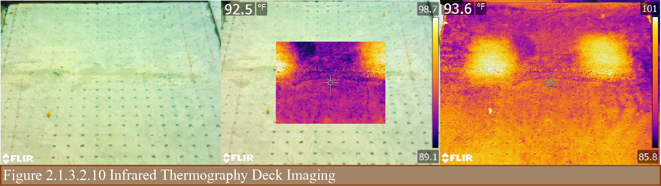
Condition data for bridges is normally collected by visual means supplemented by simple hand held devices including sounding tools (hammers) to determine material integrity, dimensional measurement tools (rulers, calipers, etc.) to determine corroded steel remaining thickness, crack dimensions, displacements, etc., and waterway probing sticks to determine integrity of soil foundation material. Advanced tools may be used to investigate known problems and vulnerabilities, or to provide more accurate assessment of phenomenon and deficiencies that are difficult to detect visually. For example, bridge decks are normally difficult to assess without interrupting traffic, and are commonly composed of reinforced concrete, a material type whose defects may not be detected by visual means. Some owners are using vehicle mounted infrared thermography or ground penetrating radar to assess bridge deck condition. This data collection can proceed at normal roadway travel speeds and produce sufficient data to identify early prevention treatment needs, determine the most cost effective work action for decks (preservation, rehabilitation, or replacement), or assist in future planning and budgeting.
Infrared thermography assessment measures temperature variations across the surface of an object. Radiated temperature variations result from differences in thermal conductivity, specific heat capacity, and mass density (Figure 2.1.3.2.10). When solar radiation heats up a bridge deck, the absorbed energy is gradually emitted. Delamination, voids, and other anomalies have different properties than the surrounding concrete and will emit different radiation. Infrared thermography performs well identifying locations of horizontal cracking or voids. The two predominant modes of bridge deck deterioration result in horizontal cracking or planar voids. Corrosion of multiple and adjacent bridge deck reinforcing steel bars results in delamination which is horizontal planar cracking induced by steel volume increase from corrosion. Bridge deck rigid overlay deterioration often starts as debonding from the deck substrate which appears as horizontal voids. Infrared thermography surveys are conducted using infrared cameras in combination with conventional video imaging. A manual review of the images is then performed to estimate location, magnitude, and severity of deterioration which shows up as locations of greater emittance.
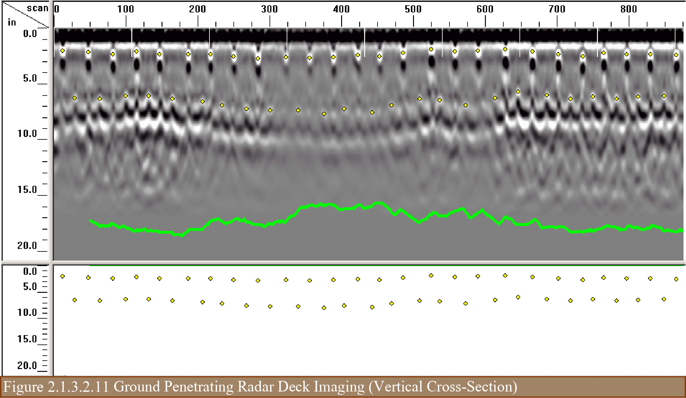
Assessment by ground penetrating radar involves transmitting electromagnetic waves and measuring the reflections (Figure 2.1.3.2.11). The amplitude, frequency, and properties of the reflected waves are dependent on the material properties. A portion of the energy is reflected from material differences, interfaces, and discontinuities. The deck surface, reinforcing steel surface, and large voids are the predominant reflectors. Ground penetrating radar does not perform as well as infrared thermography at identifying deck delamination and overlay debonding, but it performs well mapping reinforcing steel depth and assessing the potential for concrete deterioration and delamination. The attenuation of the signal at the level of reinforcing steel is normally used to represent the condition of the deck. When an antenna is centered directly above the steel, the highest amplitude return is obtained. This amplitude will be highest when the location is in good condition and lowest when corrosion and delamination is present. The technology requires specialized expertise for data collection and post processing for correct interpretation of results. Similar to infrared thermography, the data can be used to estimate location, magnitude, and severity of deterioration.
It is important to ensure the quality of data during its collection. Quality control and assurance is important during all stages and processes including pre-survey calibration, during the survey, validation, daily checks, continuous monitoring of equipment and results, correct processing, and the storing and securing of data.
A detailed quality management plan (QMP) should be prepared for the data collection. The QMP is expected to ensure that the acquisition of the required data meets the road organization’s needs and specifications. The QMP has to address, among other considerations, the following issues:
Condition indices describe a set of discrete, ordered states determining the rating of asset condition parameters. Trained condition rating personnel may assess the current state of the asset and assign a rating to that asset. However, the subjective rating can vary by rater.
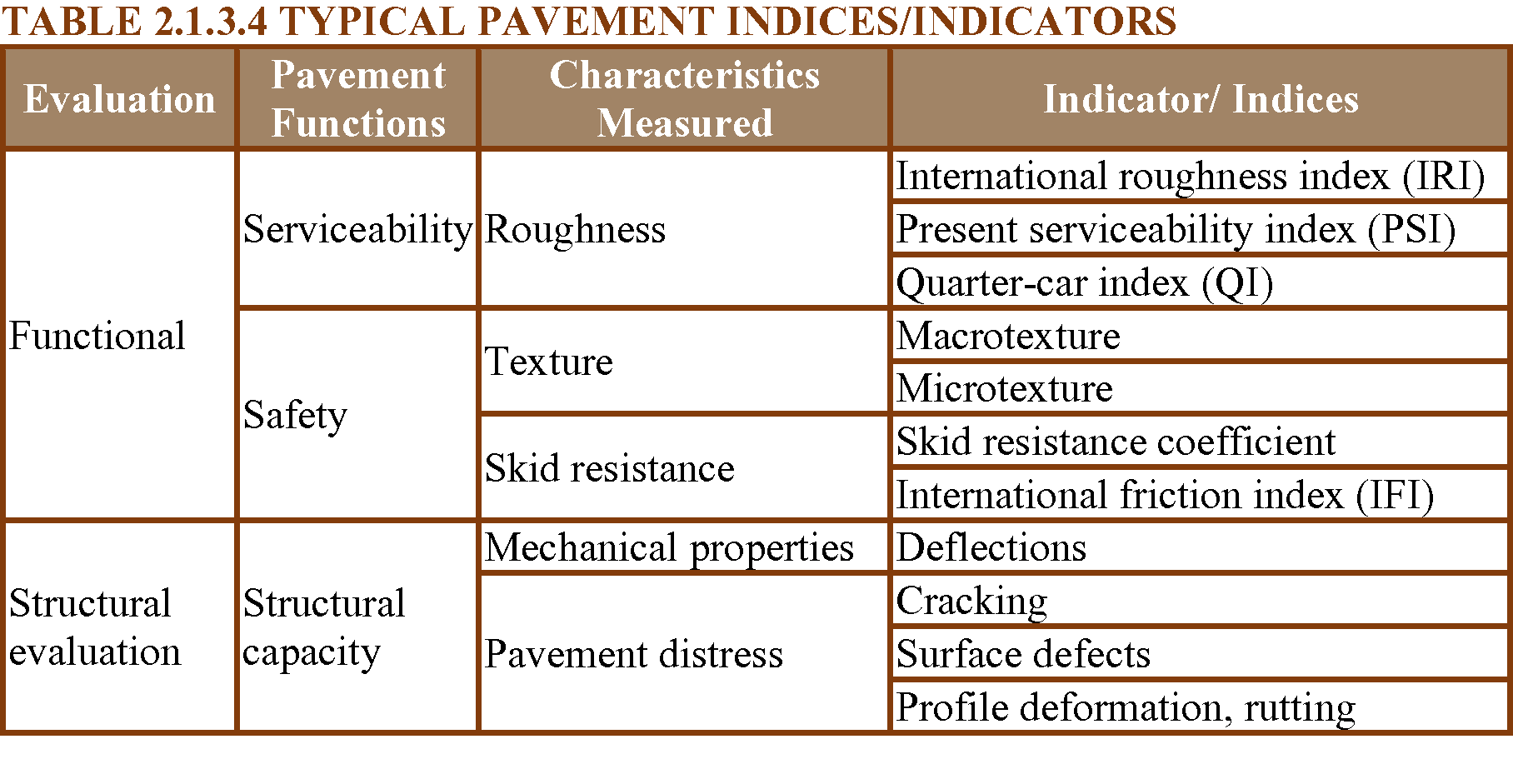
The pavement conditions normally evaluated for asset management are as follows:
The above characteristics are measured in the field by acceptable equipment and methodologies and are quantified by means of indicators or condition indices. Typical pavement condition indicators and indices are shown in Table 2.1.3.4.
Bridge condition indices are typically represented by condition states of individual elements that are then combined in to component rating, e.g. deck rating and then an overall bridge condition index (BCI).
Bennett 1999. Bennett, C.R. and Paterson, W.D.O. Guidelines on Calibration and Adaptation, HDM-4 Technical Reference Series, Volume 5.
Bennett 2007. Bennett, C.R. et al. Technologies for Road Management, Version 2, The World Bank.
Birmingham 2002. University of Birmingham/Transit NZ. Road Asset Management Principles.
Flintsch, G. W., & Bryant, J. W. (2006). Asset management data collection for supporting decision processes. US Department of Transport, Federal Highway Administration, Washington, DC. (https://www.fhwa.dot.gov/asset/dataintegration/if08018/assetmgmt_web.pdf).
OECD 2001. Asset Management for Road Sector.
PIARC 2003. Automated Pavement Cracking Assessment Equipment - State of the Art, Committee on Road Pavements, ISBN: 2-84060-156-7 (https://www.piarc.org/en/order-library/4407-en-Automated%20Pavement%20Cracking%20Assessment%20Equipment%20-%20State%20of%20the%20Art.htm)
PIARC 2004. Asset Management in relation to Bridge Management, Committee on Bridges and Other Structures (11), ISBN: 2-84060-167-2 (https://www.piarc.org/en/order-library/4414-en-Asset%20Management%20in%20relation%20to%20Bridge%20Management.htm).
PIARC 2005. Asset Management for Roads - An Overview, Committee on Road Management (C6) (https://www.piarc.org/ressources/publications/2/4545,06-09-VCD.pdf).
PIARC 2006. Asset management of Honshu-Shikoku bridges (https://www.piarc.org/ressources/publications/8/24326,Ponts-Routiers-Revue-Routes-Roads-Magazine-369-Road-Bridges-World-Road-Association-Mondiale-de-la-Route-064.pdf).
PIARC 2011. Large Road Bridges: Management, Assessment, Inspection, Innovative Maintenance Techniques, Technical Committee D.3 – Road Bridges. ISBN: 2-84060-239-3. (https://www.piarc.org/ressources/publications/6/11606,2011R06.pdf).
PIARC 2018. The Use of Unmanned Aerial Systems for Road Infrastructure, 2018SP03EN. (https://www.piarc.org/ressources/publications/10/29479,2018SP03EN.pdf).
Telli 2010. Telli Van der Lel et al. Evaluating Asset Management Maturity in the Netherlands.
UK Roads 2013. UK Roads Liason Group. Highway Infrastructure Asset Management.
USDOT 2018. U.S. Department of Transportation, Federal Highway Administration Nondestructive Evaluation Web Manual (https://fhwaapps.fhwa.dot.gov/ndep/TechnologyMenu.aspx).
World Bank 1997. Selecting Road Management Systems (http://documents.worldbank.org/curated/en/196321468762908116/pdf/multi-page.pdf).
The following case studies are presented in this chapter:
CASE STUDY 1: Implementation of Road Asset Management and Inventory Systems for the state roads of Pahang, Malaysia – Data collection
CASE STUDY 2: Road inventory and automatic visual inspection in Chile
CASE STUDY 3: Inventory, inspection and reporting of dynamic traffic management sign gantries at Flemish Roads and Traffic Agency (AWV)
The state government of Pahang, Malaysia, decided to implement a road asset management system for its state road network as part of a long-term road maintenance contract of seven years with a private company appointed in April 2013. The company was to maintain 2,300 km of the state road network and implement a road asset management system. The scope of road maintenance work included routine maintenance, periodic maintenance, and emergency maintenance. The contract also included the provision of an asset management system (YP-RAMS) and a road asset inventory management system (YP-RIMS).
The data collection for the asset management system involved the collection of road asset inventory data and a pavement condition survey to be carried out for the entire network in the first year. The collection of road asset inventory data and a pavement condition survey for 30 percent of the network was to be carried out from the second year until the end of the contract period. The use of GPS coordinates and digital recording for all asset points and referencing was compulsory. The road asset inventory management system needed to be updated and inventory reports produced every year. The new road asset management module needed to be inter-phased or integrated into a pavement management system, geographic information system (GIS), road asset inventory management system, and road inventory and road condition database.
The asset management software system makes use of a common inventory and database on the ArcGIS platform. The network condition data are measured in accordance with the International Roughness Index (IRI), cracks, and pavement strength. Digital recordings of the -of-way were taken for the entire network. Traffic data were collected from selected traffic count stations in terms of AADT and axle loading.
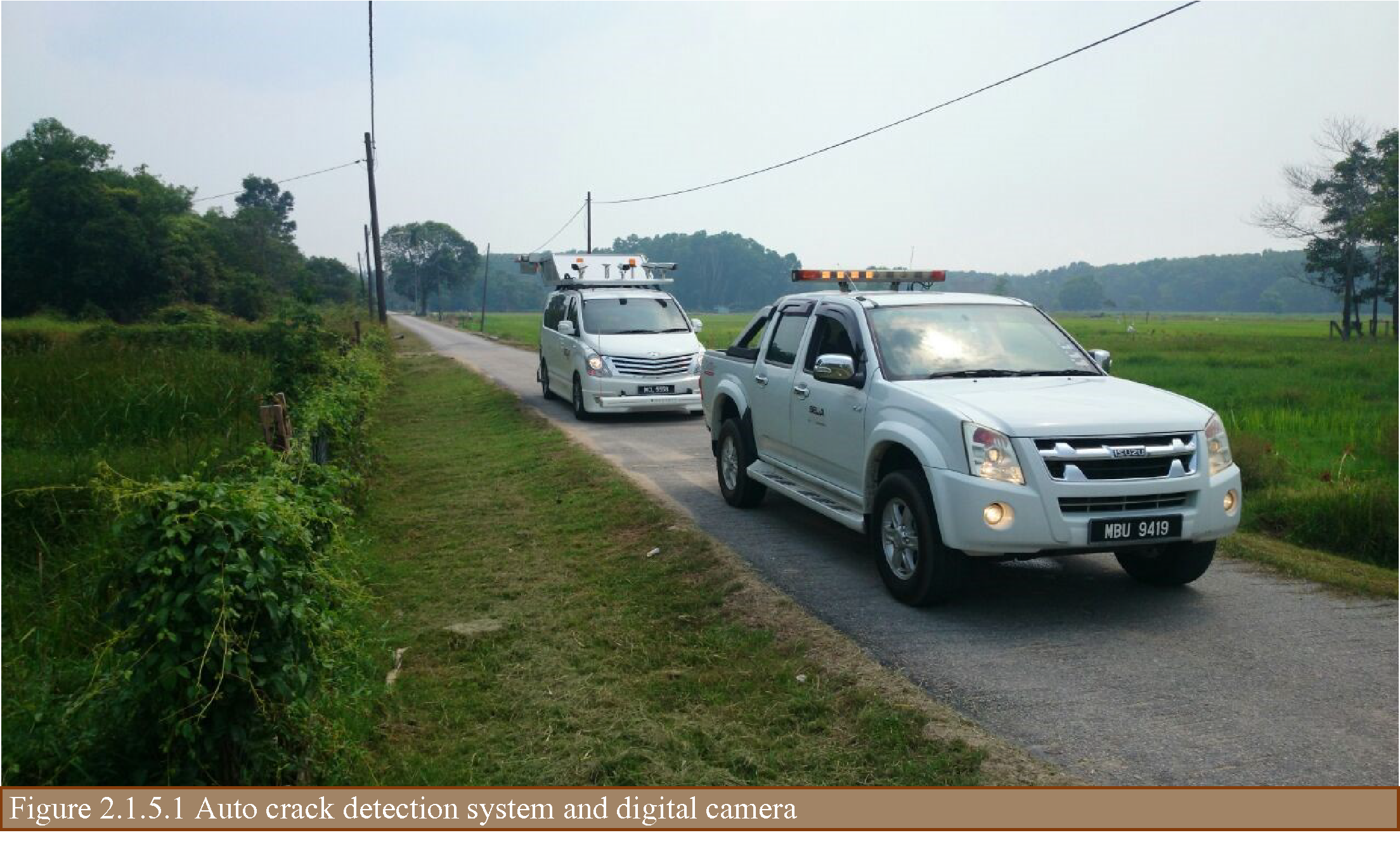
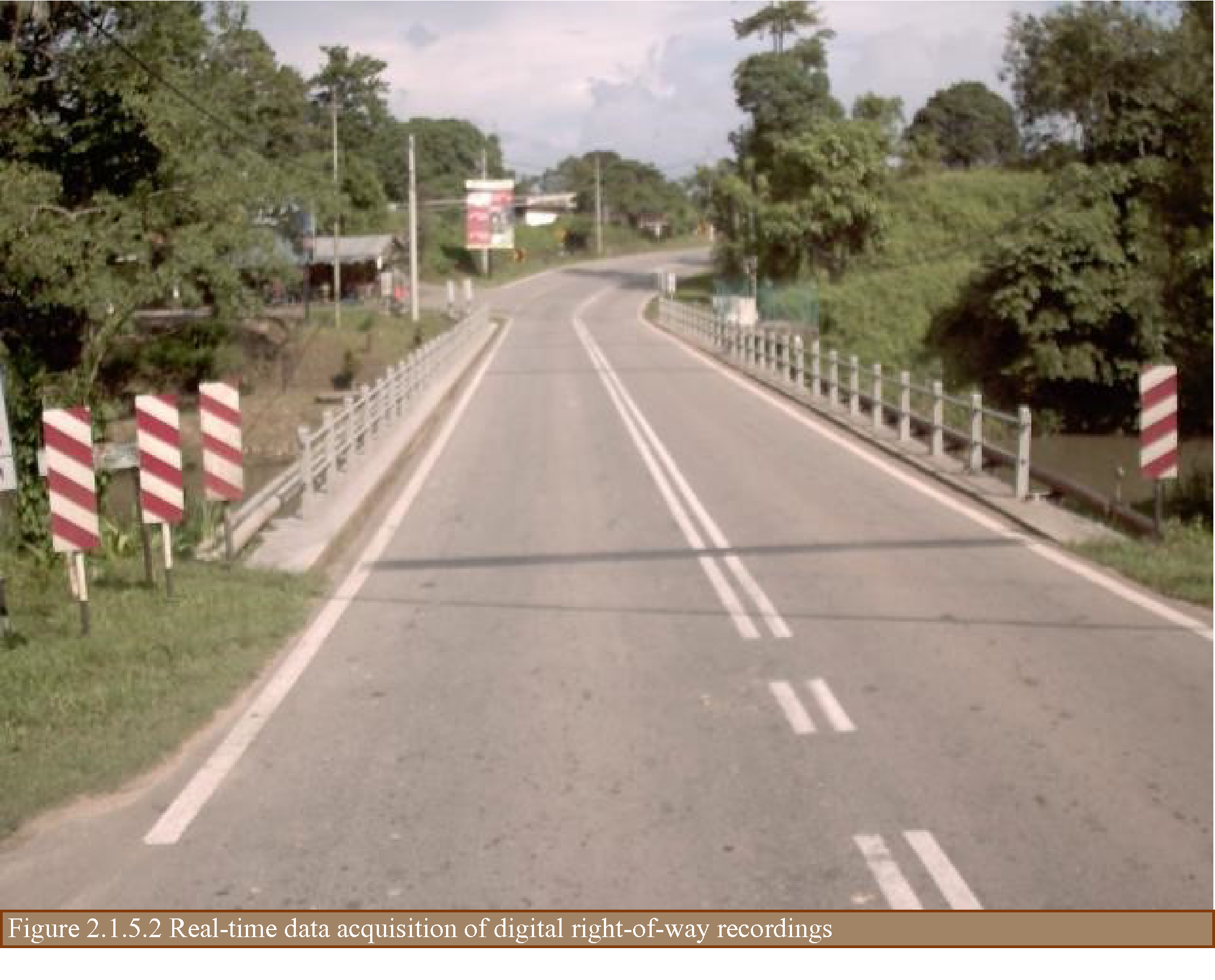
The project managers opted to outsource the data collection equipment rather than purchase new equipment. This proved to be cost-effective, considering the idle time between data collection intervals. The techniques and equipment used included a multi-laser profiler and automatic crack detection (ACD) system, FWD, asphalt coring, and a dynamic cone penetrometer. The techniques and equipment used are shown in Figures 2.1.5.1 and 2.1.5.2 The following data were collected:
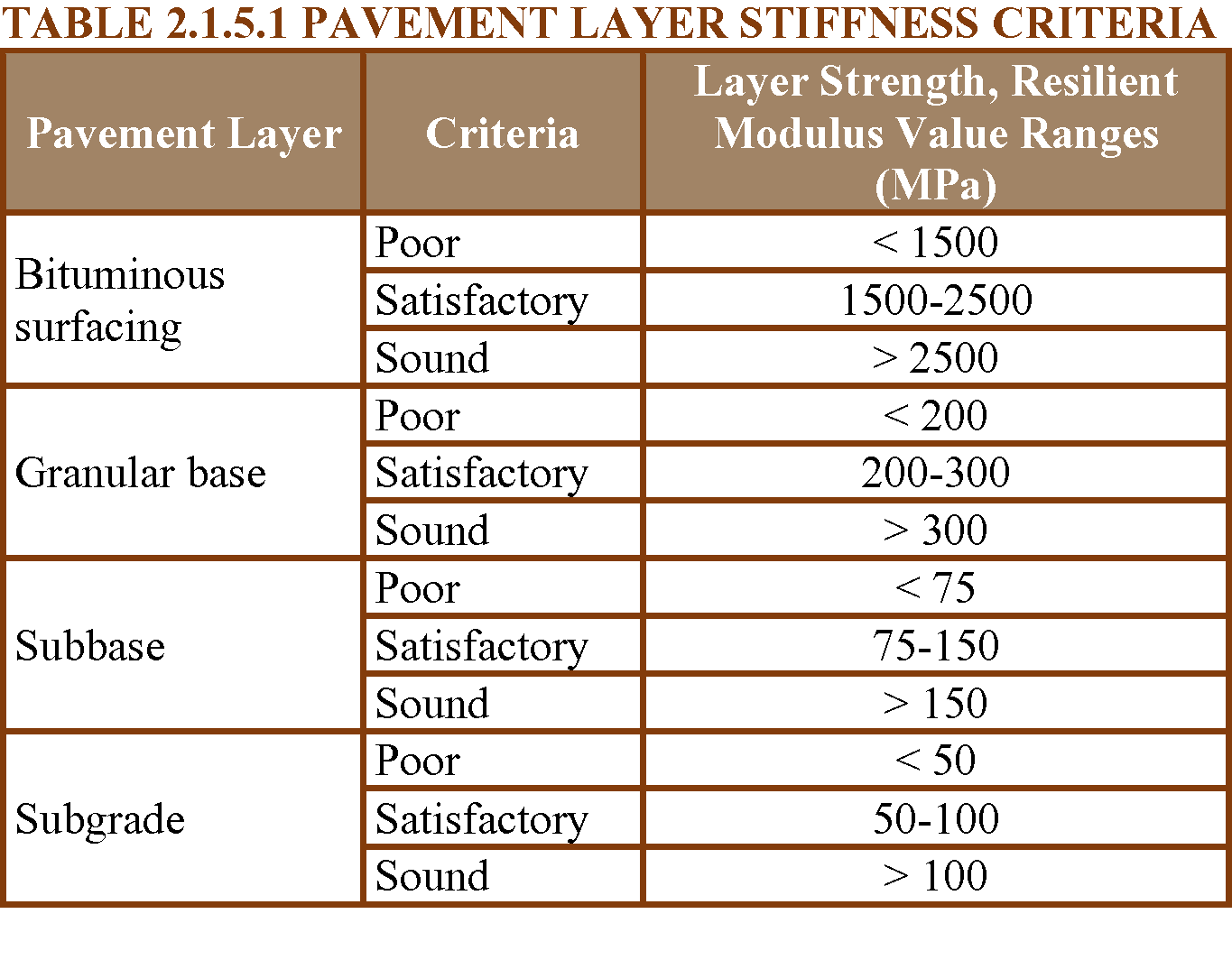
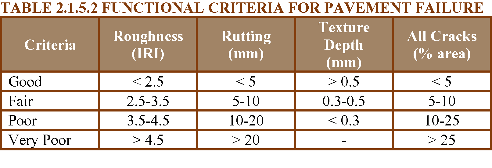
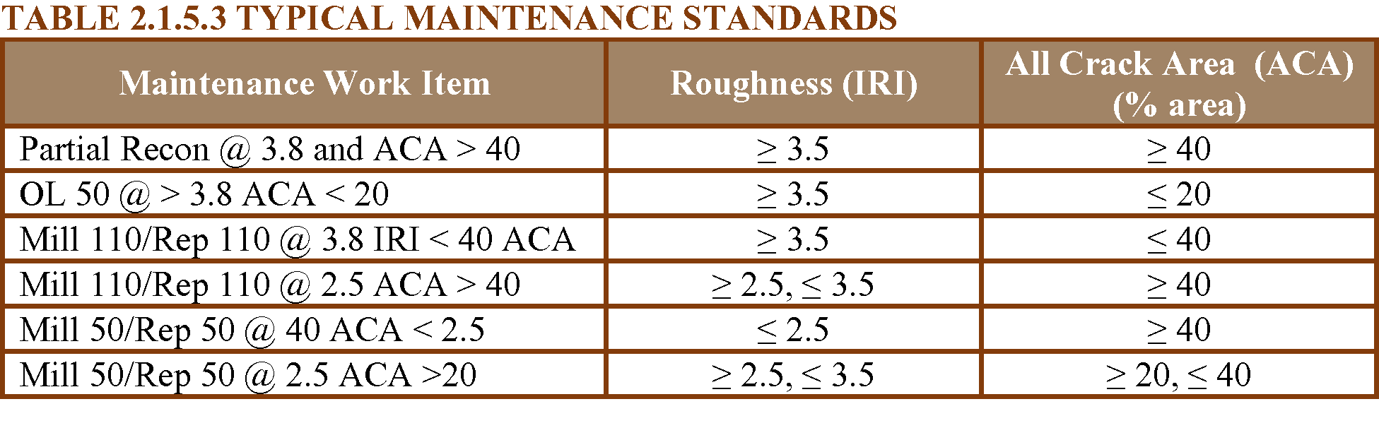
The criteria used for data collection and analysis are shown in Tables 2.1.5.1 to 2.1.5.3.
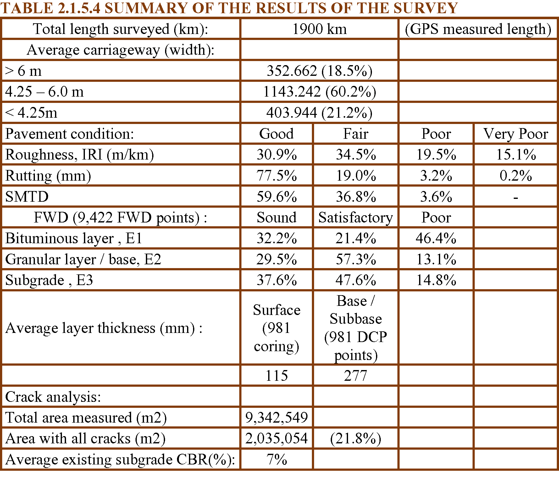
The collected road data were processed using the respective software of the equipment used. A summary of the outcome of the surveys is shown in Table 2.1.5.4.
HDM-4 (Bennett 1999, 2007) was used to evaluate the maintenance requirements based on the maintenance standard specified. With the base year 2014, the predicted cost by each district is shown in Figure 2.1.5.3.
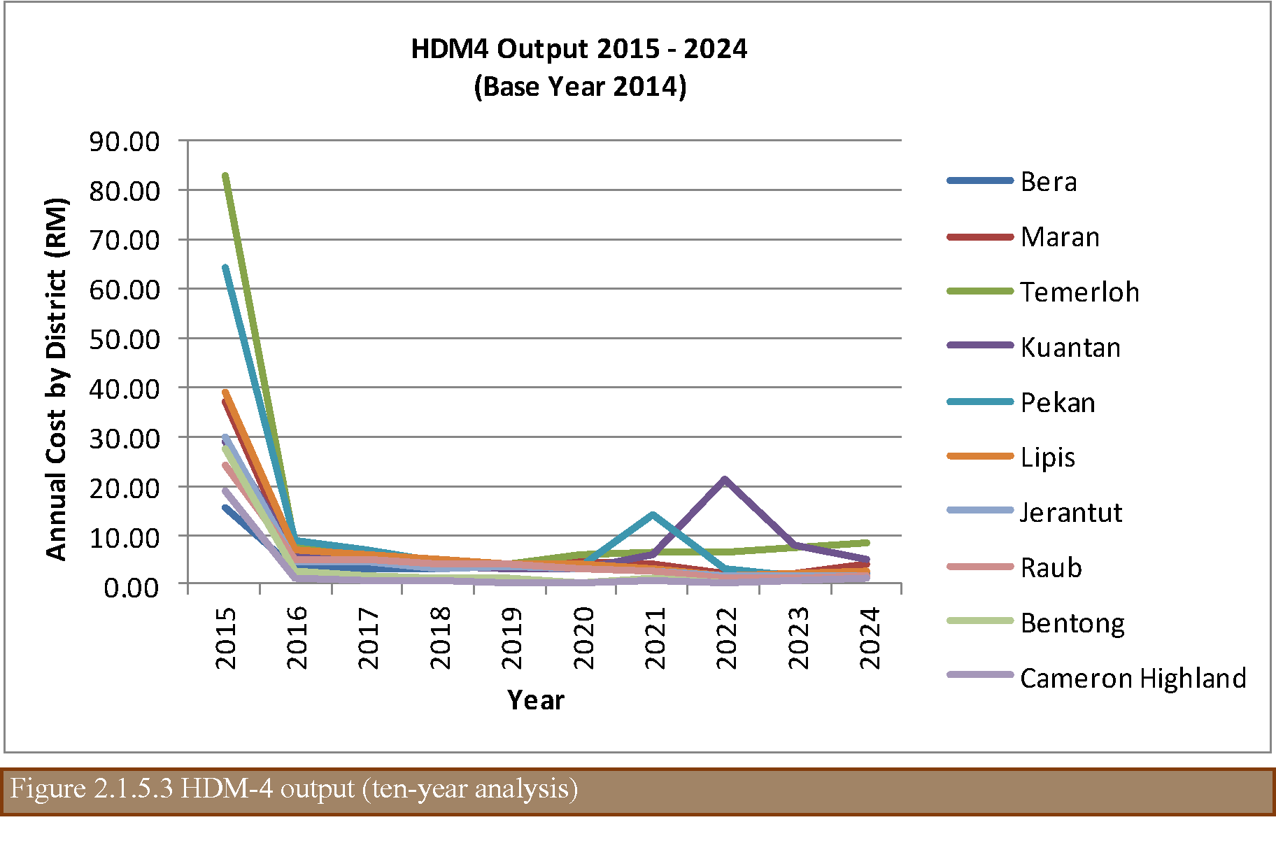
In conclusion, the proper and systematic collection of data using the correct and appropriate data collection equipment allows an adequate maintenance strategy to be applied.
CARLOS RUIZ TREVIZAN, National Highways Laboratory Department, Highway office, Chile
In recent years in Chile, activities have been intensified to improve traditional road maintenance management systems, innovating and diversifying the management systems of road conservation activities, incorporating road network systems, service levels, road concessions, execution and maintenance of basic roads (low cost roads) and maintenance by Direct Administration (using its own personnel and resources of the National Road Directorate of Chile).
One of the main axes to support this sustained growth in road management currently in Chile is the information provided by the Road Inventory and Visual Inspection of Paved Roads, which is done through automated equipment. This equipment with digital cameras, bars with lasers and bars with geophones are mounted on a vehicle which travels on the road at the same speed of flow and collects much of the information that is needed. IRI data can be obtained, cracking, road geometry, signaling, lighting, road safety, demarcation and shoulder data, among other parameters. The data is stored immediately and can be transferred to any database format required by the network administrator (see Figure 2.1.5.4).

The captured and georeferenced digital images are entered into a program to identify the types of deterioration present in the roadway and a severity is assigned to then compute the deteriorated areas. The structural and functional deteriorations are then entered into the ICP indicator (Pavement Condition Index) to determine the qualitative and quantitative condition of the pavement. The ICP indicator corresponds to an own design of the Road Directorate of Chile and is the product of an extensive and complete study of behavior of the pavements, framed this in the implementation of a robust system of management of the pavements.
Another technology that has gone in breakthrough is the Georradar, which is a non-destructive technique that is based on the emission and propagation of electromagnetic waves in a medium, with the subsequent reception of the reflections that occur in their discontinuities. The application in a first stage of 5,500 kilometers of pavements, complemented with the extraction of witnesses of pavements and exploration shafts on the side of the roads, allowed to update and correct a large part of the road inventory of paved roads in terms of characteristics and types of materials that make up the road surface.
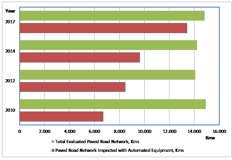
Currently in Chile, and after several periods performing the visual inspections of pavements by manual means and with personnel from the National Road Directorate itself, it has been decided for 4 consecutive periods to carry out a large percentage of this task through consulting contracts and with automated means. In 2017 they were tendered in the National Roads Authority of Chile 13,404 kilometers of automated auscultation of about 14,834 total kilometers evaluable, representing 90.4%. This growth in the automated visual inspection of pavements carried out in Chile can be seen in Figure 2.1.5.5.
With the results of this automated visual inspection, a large amount of parameter information is obtained from the paved network, which allows the execution of the HDM-4 software to develop periodic maintenance projects that maximize social benefits and provide a greater social return of investment in the country's road infrastructure. These projects are proposed to each of the 16 Regional Road Directions in which the country is administratively divided to be considered in the prioritization of the works that will be executed in the short term and in the relevant budgetary processes. In addition, the automated visual inspection allows tracking the status of the paved road network of the country so that the community and the authorities of the country have a global knowledge of its evolution as shown in the following Figure 2.1.5.6:
This summarizes the activities and results obtained from the process described above, which is currently carried out in Chile to manage the entire paved network under the responsibility of the National Roads Department. More information on this can be found on the website of the Roads Department of Chile according to the link: http://www.vialidad.cl/areasdevialidad/gestionvial/Paginas/Informesyestudios.aspx
BEN HELSEN, Flemish Roads and Traffic Agency (AWV) - EMT, Belgium
The IIR (Inventory, Inspection and Reporting) project was started within the Flemish roads and traffic agency (AWV) in 2012, with a view to achieving efficient inventorying and inspection of road accessories (both electrical equipment and the actual road accessories, as well as road condition).As part of the group of electromechanical facilities, sign gantries for dynamic traffic management (DTM) were included in the project from the start, mainly on account of their potential risk (position above the carriageway).
The electromechanics and telematics (EMT) division of AWV – more specifically its traffic enforcement systems (VHS) team, which also provides the operational management of those facilities – was placed in charge. The objective of AWV is to take a detailed inventory of the full asset in place. Newly installed facilities (e.g. in new construction projects) are added to the inventory as standard procedure.
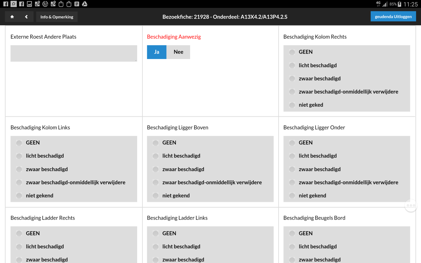
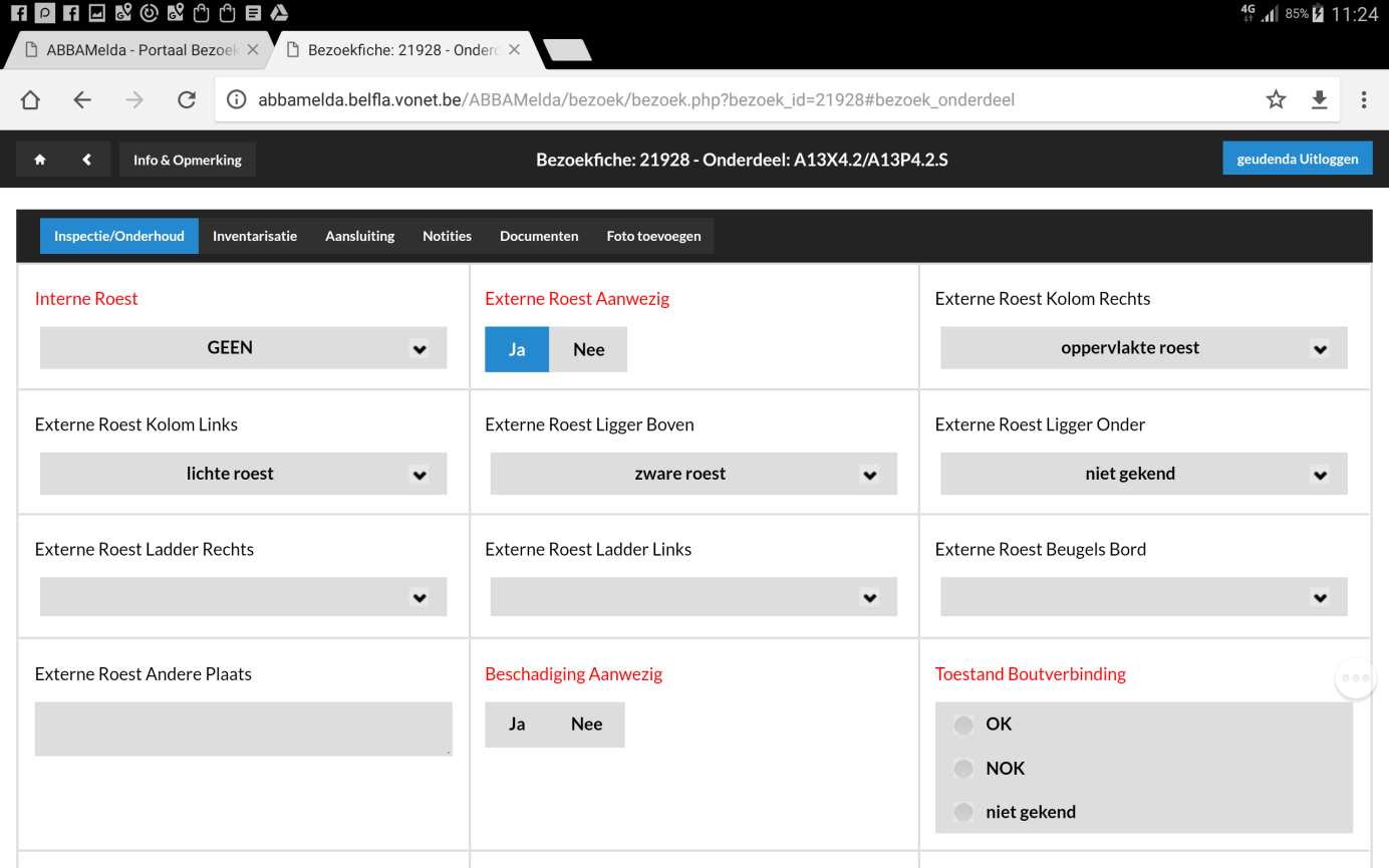
The inspections include assessing and recording the condition of the facility, with special focus on stability, corrosion and the condition not only of the columns, but also of the clamps and bolts.
The approach is a basic solution to manage the maintenance risk of electromechanical facilities, sign gantries for dynamic traffic management (DTM) on the Flemish roads.
Efficient inventorying and inspection of road accessories. The objective of AWV is to take a detailed inventory of the full asset in place.
The inspections include assessing and recording the condition of the facility, with special focus on stability, corrosion and the condition not only of the columns, but also of the clamps and bolts.
Structured detailed inventory of the asset (of DTM sign gantries in this case), with a representative inspected status of both the entire facilities and their relevant parts. Using this inventory, status reporting makes it possible not only to define an adequate maintenance policy but also to take targeted remedial (or, if necessary, proactive) measures through the maintenance programme – which is otherwise mainly directed to operationality – or, if necessary, through well-advised targeted (re-)investments.
Before the IIR project, AbbaMelda was already a first form of asset management, at least as far as the electromechanical facilities managed by AWV’s EMT division were concerned. However, it was a rather single level and little structured listing of facilities mainly intended for use in calling up the contractors concerned in case of defects or damage and in recording the calls and their handling. Moreover, the listing was high-level as far as the facilities were concerned, with little on no specification of component parts and, consequenly, few or no interrelations.
A safety incident triggered the setting up of the IIR project, which built on the existing AbbaMelda data base for electromechanical facilities such as DTM sign gantries.
The facilities already included were renamed in many cases, but also – and mainly - often merged into coherent logical sets. Many more component parts were specified and included (e.g., not only the sign gantry with variable message signs, but also the individual signs, their controller cabinet and the representative parts inside, and characteristics of, that cabinet. Electric power supply and the communication network were included as well.
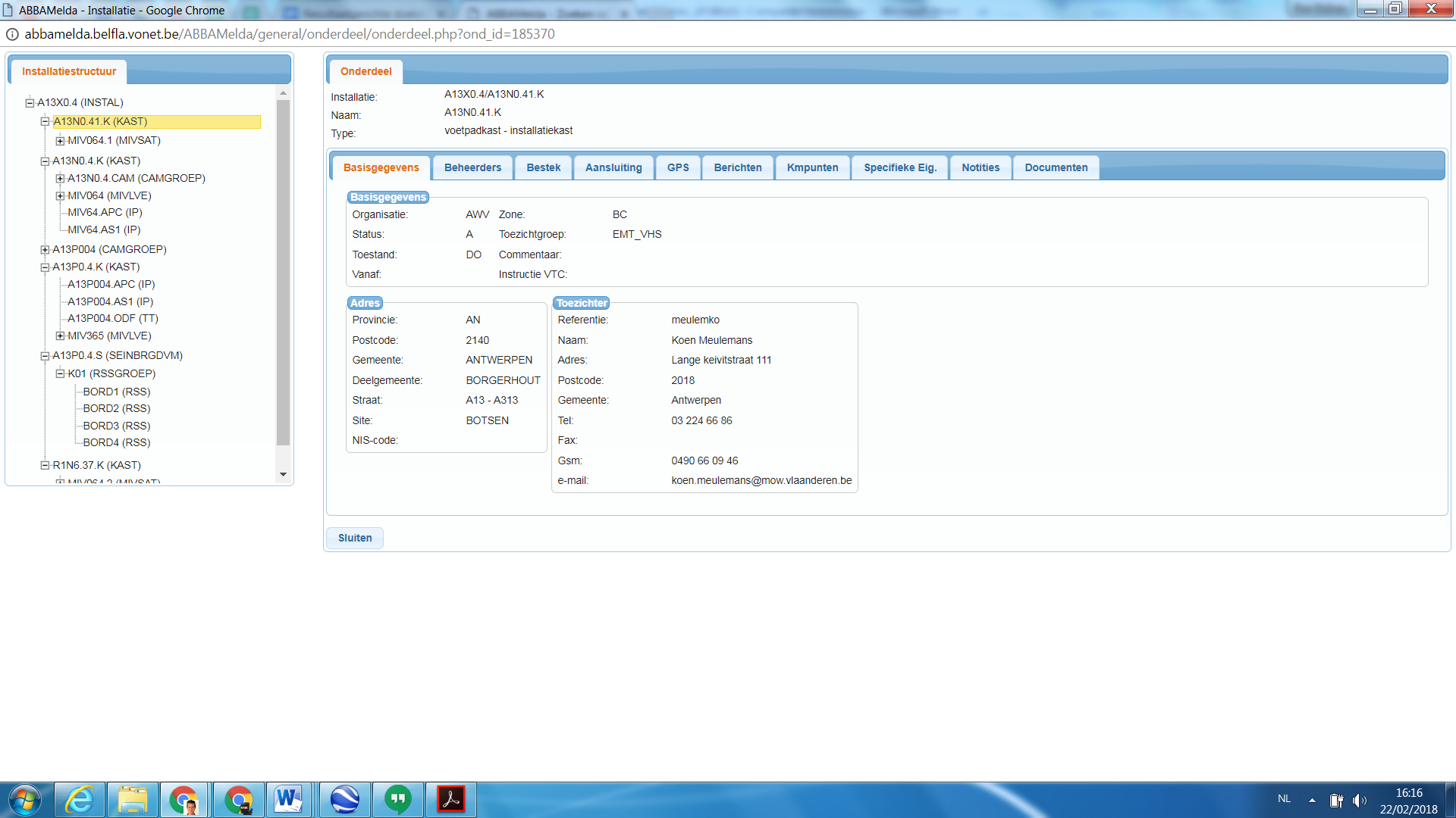
Additionally, maximum accuracy (typically GPS) location data were assigned to the facilities and parts, enabling the data to be coupled in numerous GIS applications for various purposes (e.g., conflict detection in case of scheduled works).
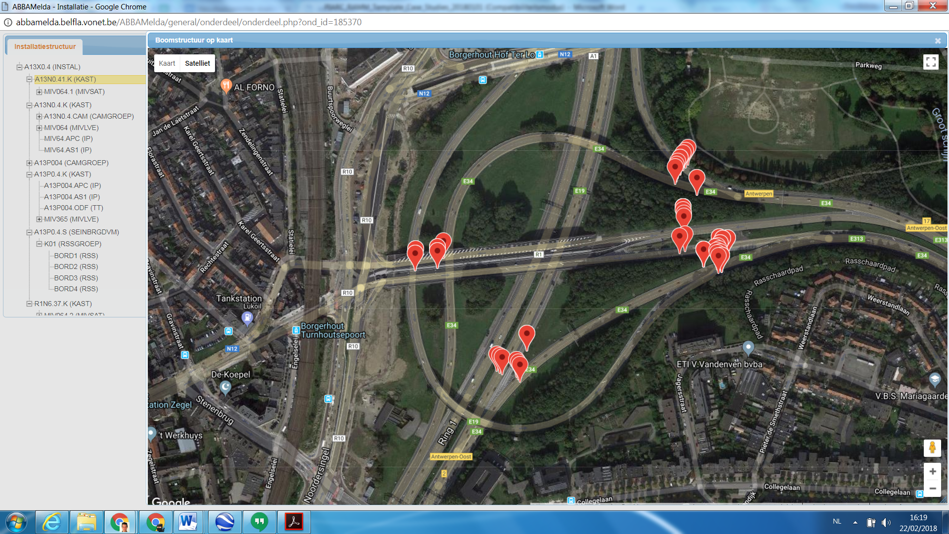
Figure 2.1.5.8: AbbaMelda data base for electromechanical facilities
A portal named “Mobiel” was developed for use on a tablet, which made it possible not only to inventory (or continue inventorying) facilities on site, but also, and mainly, to inspect them.
A few screenshots for DTM sign gantries are presented below.
Two new projects were recently started. In the first project, the existing application AbbaMelda is divided into two parts, with the facility database part being renewed into a modern application which not only better suits the functional needs but wil also, and mainly, provide additional possibilities for interrelations, structures, etc. Concurrently, an AIM/BIM-oriented project was launched at AWV level.
Whereas a few years ago AbbaMelda was mainly a tool for recording and monitoring defect repairs, it has developed and is still developing further into a central data base of electromechanical facilities managed by AWV: type of facility, location, interrelations, status, parts, persons in charge, etc.
The process and procedure of monitoring and reviewing the performance of asset management and the performance and/or condition of assets is presented in this chapter, which provides answers to the following questions:
Performance monitoring is the process of monitoring and reviewing the performance of asset management and the performance and/or condition of assets.
The performance framework discussed in section 1.4 creates a top-down connective thread from organizational direction and goals down to individual, day-to-day management activities (PIARC 2004). Similarly, the bottom-up monitoring of performance (asset characteristics, management systems problems, risks and opportunities) should provide the factual basis for adjusting and refining realistic asset management strategies and plans, through a process of continual improvement.
Therefore, the organization should establish, implement, and maintain processes and/or procedure(s) for the following:
This process is not intended to replace audit processes that may already be in place.
The performance monitoring process should cover the following areas (HMEP 2013, CSS & TAG 2004):
Strategic monitoring: To verify that outcomes are being met and asset management has been implemented and documented.
Performance measures and targets: To assess the effectiveness and efficiency of asset management.
System audits: To review and evaluate the effectiveness of asset management retrospectively (e.g., on an annual basis).
Compliance monitoring – To evaluate the organization’s compliance with applicable legal and absolute or regulatory requirements.
Performance Monitoring is the process and procedure of monitoring and reviewing the asset management framework
Frequency of monitoring should find the balance between the cost of collecting the monitoring data and information and the risks of not having the information available. Finding the balance is particularly important when considering compliance with statutory obligations and demonstrating value for money.
It is also important that the benefits from implementing asset management are captured and measured against those identified in the case for investment, or to support value for money initiatives or greater efficiency in delivery of the service. Recording and demonstrating the benefits may provide essential evidence for further investment. Demonstrating benefits is therefore a key success factor in the implementation of asset management and should form part of the monitoring process.
Monitoring and reporting performance (PIARC 2002) is an important part of demonstrating whether the organization is delivering the agreed levels of service (NAMS Group 2011).
The measurement of organizational performance provides the following:
Information and data arising from the implementation and delivery of asset management provide the following:
This information will also enable critical issues regarding performance to be identified and improvement plans to be developed.
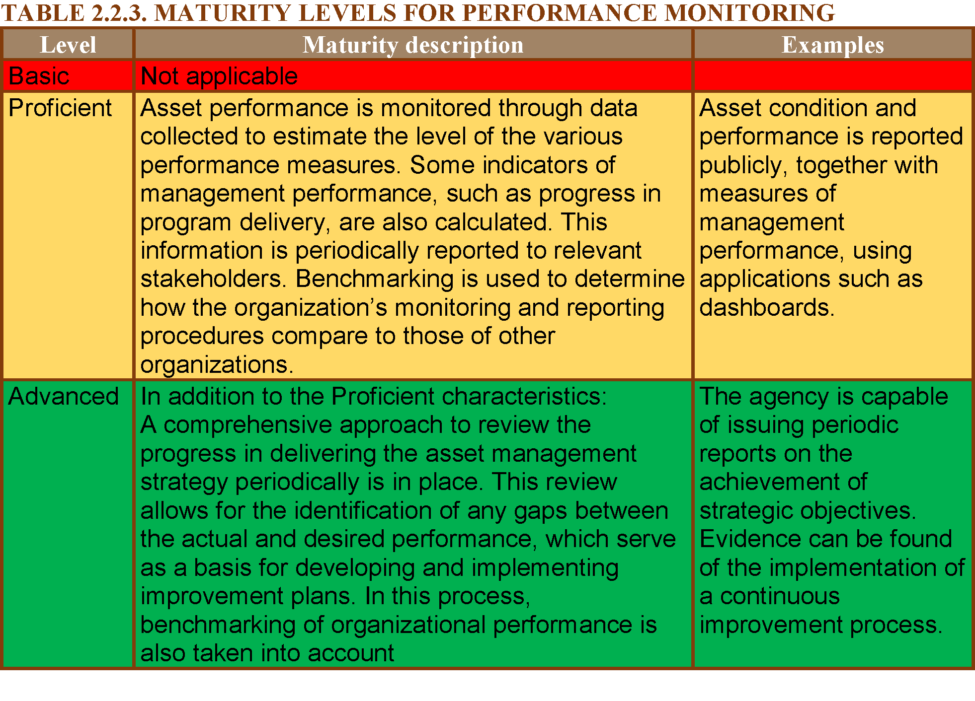
In terms of performance monitoring, Asset Management maturity levels can be defined as shown in table 2.2.3.
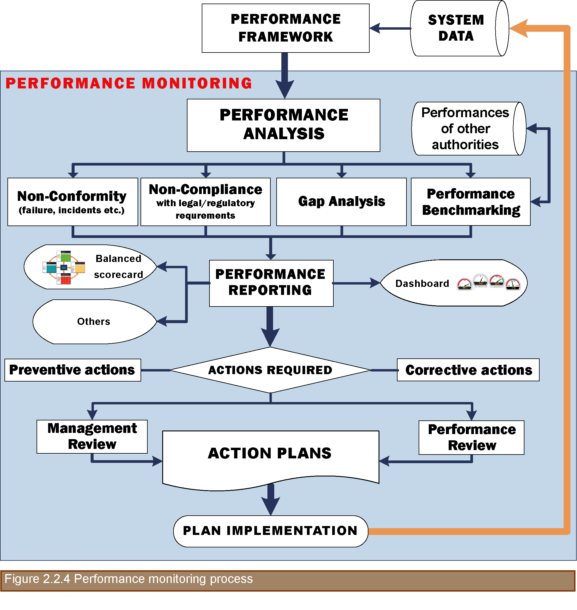
During the implementation of the asset management plan, the performance of the asset management plan and the performance and/or condition of assets and/or asset systems are assessed through collecting information and data (see section 2.1) and evaluating levels of service as defined in the performance framework (see section 1.4). Measuring current performance, which should be reported through various means, allows the organization to compare actual and expected performance by identifying any existing gaps. Gap analysis, in conjunction with performance reviews and benchmarking, are used in determining actions to be implemented if the current performance falls below the organization’s requirements or if ways to improve the efficacy and efficiency of the asset management approach are identified. The performance monitoring process is depicted in figure 2.2.4.
A performance gap in the monitoring process is the difference between the current performance of an asset and the expected performance reported in the management plan.
There are a number of ways in which performance measures can be summarized and reported. In deciding upon a reporting format, considerations should be given to the following:
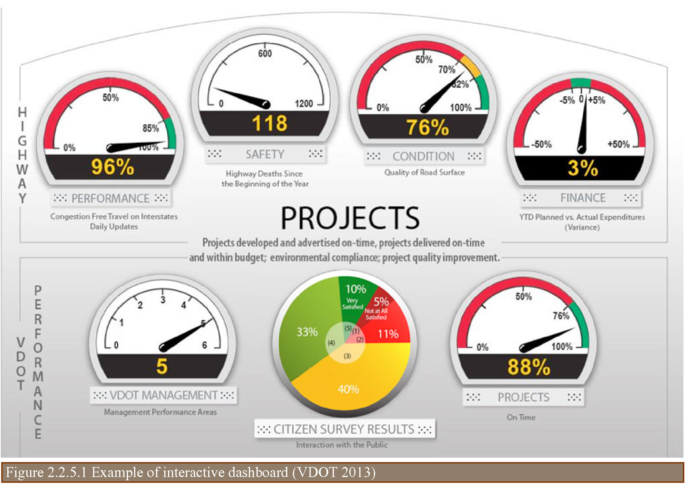
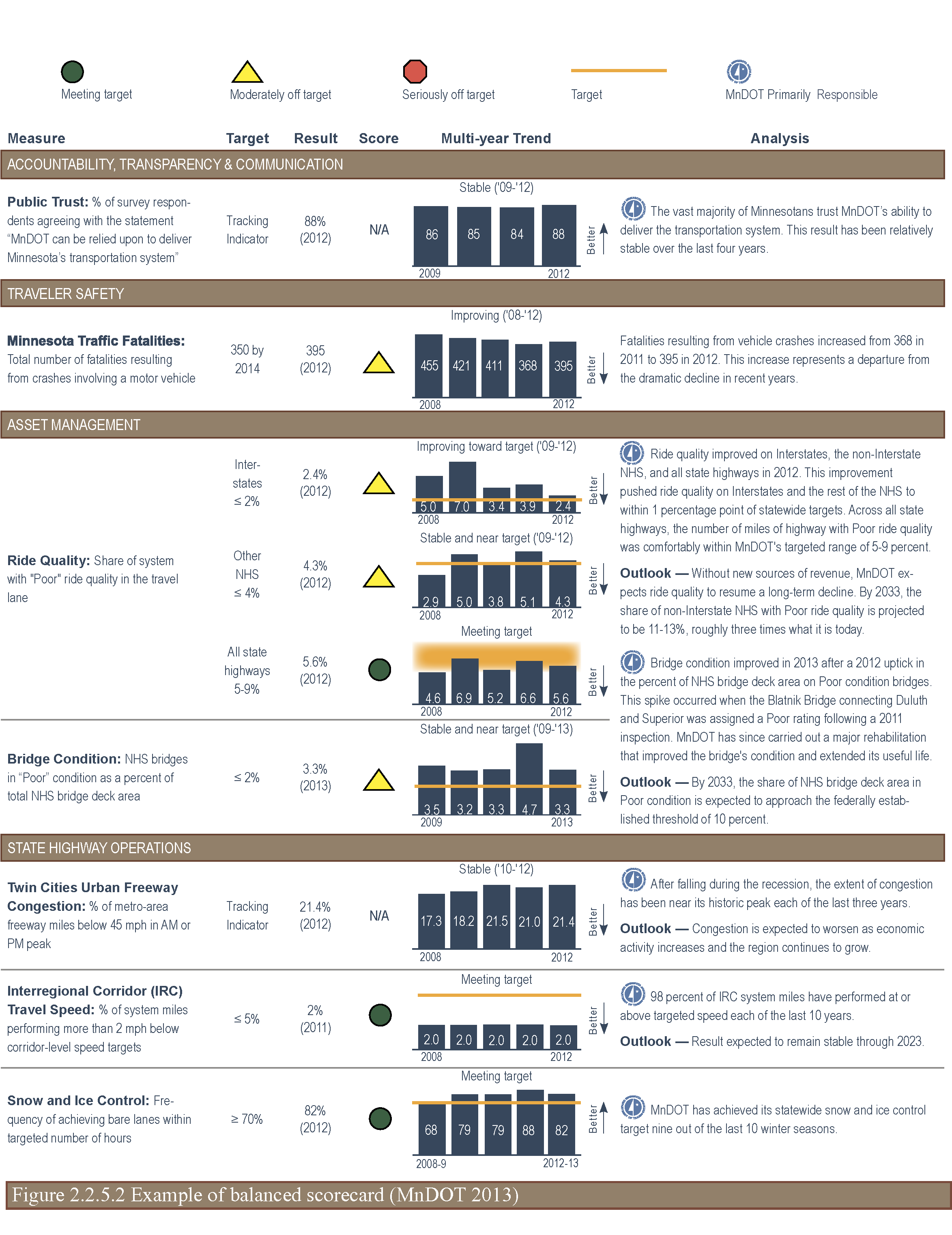
At present, there is an increasing demand for organizations to report not only financial and service outcomes, but also the social and environmental effects, and to demonstrate to stakeholders and political authorities that the organization is managing their social and environmental responsibilities (PIARC 2003). In this case, the balance scorecard and the dashboard approaches, described below, are appropriate as tools for demonstrating the level of attention given to each outcome area among competing demands.
The balance scorecard and dashboard techniques use technical, non-technical, economic, and financial performance measures, normally less than 25, spread across two or more “themes” or “perspectives” (see examples in figures 2.2.5.1 and 2.2.5.2).
At the proficient level of service, performance measures related to the strategic objectives of the agency are normally reported at all organizational levels and to customers in an appropriate form (often via an annual report) (NAMS Group 2011).
As previously noted, performance monitoring is an element in a cycle structured to support a process of continuous audit and review of the plan and the processes used. Therefore, information from the performance monitoring and reporting processes should be used to review the asset management approach. Review activities may include the following:
The performance review involves the consideration of results, the factors contributing to performance, and options for dealing with substandard outcomes; it is carried out at regular intervals, usually on annual basis.
The management review involves an assessment of the need for changes to the asset management framework, including asset management policies, strategies and objectives (PIARC 2017). The outputs from the management review may include changes in policies, strategies, and objectives; performance requirements; resources; or other elements of the asset management approach. Some of these outputs may also generate changes in the organization’s strategic plan. Plans are normally reviewed and updated every three years because this time is considered long enough for the action indicated by the original plan to have taken effect.
The purpose of benchmarking is to compare the organization’s own asset management practices against those of a selection of similar organizations, but it is important that the comparison takes into account the organization’s overarching context and circumstances. Benchmarking should be seen as a positive and proactive process whereby an organization assesses how it performs activities in comparison to other organizations.
Four approaches to benchmarking may be considered, each of which provides a different perspective:
As a result of any of the reviews, organizations are likely to identify a series of desirable improvements they wish to put in place in order to advance their asset management practice. These improvements may be formally documented in an action plan. The plan should not only detail the specific actions to be taken, but also outline which levels of service the actions are intended to benefit. Furthermore, in developing the improvement plan, it is important that organizations be pragmatic about what can be delivered given the likely staff resources and budget.
Actions should be prioritized and placed into timeframes, and they can be classified as corrective or preventive, as follows:
County Surveyor’s Society (CSS) and Transport Analysis Guidance (TAG). 2004. Framework for Highway Asset Management. Last Accessed May 2015. http://www.ukroadsliaisongroup.org/en/utilities/document-summary.cfm?docid=9E4BA1A6-74B2-414B-81205FAC797615D1.
Minnesota Department of Transportation (MnDOT). 2013. Minnesota 2012 Transportation Results Scorecard. Last accessed July 27, 2015. www.dot.state.mn.us/measures/pdf/2012-scorecard.pdf.
New Zealand National Asset Management Support (NAMS) Group. 2011. International Infrastructure Management Manual. Wellington, New Zealand.
PIARC 2003. Evaluation of Transport Performance Measures for Cities, Technical Committee 10 – Urban Areas, ISBN: 2-94060-160-5 (https://www.piarc.org/ressources/publications/2/4422,TM10-14-VCD-e.pdf).
PIARC 2004. The framework for performance indicators, Comité technique 6 Gestion des Routes / Technical Committee 6 Road Management The Framework for Performance Indicators, PIARC Paris France 2004, ISBN 2-84060-165-6 (https://www.piarc.org/en/order-library/13485-en-The%20Framework%20for%20Performance%20Indicators.htm).
PIARC 2008. Integration of Performance Indicators, Technical Committee 4.1 – Management of Road Infrastructure Assets, ISBN: 2-84060-206-7 (https://www.piarc.org/ressources/publications/4/5905,2008R06.pdf).
PIARC 2017. Management of road assets: Balancing of environmental and engineering aspects in management of road networks, : Comité technique 4.1 Gestion du patrimoine routier / Technical Committee 4.1 Management of Road Infrastructure Assets, PIARC Paris France 2017, ISBN 978-2-84060-455-6 (https://www.piarc.org/ressources/publications/9/27317,2017R05EN.pdf)
United Kingdom Roads Liaison Group (UKRLG) and Highways Maintenance Efficiency Programme (HMEP). 2013. Highway Infrastructure Asset Management Guidance Document. Department for Transport, London. http://www.ukroadsliaisongroup.org/en/utilities/document-summary.cfm?docid=5C49F48E-1CE0-477F-933ACBFA169AF8CB.
Virginia Department of Transportation (VDOT). DASHBOARD: Performance Reporting System for Projects and Programs. Virginia Department of Transportation. http://dashboard.virginiadot.org. Accessed May 2015.
DAVID K. HEIN, Applied Research Associates, Inc., Canada
In order to ensure that the condition of the roadway is adequate to maintain the usability, comfort, and safety of the travelling public, concession agreements usually include a set of conditions outlining the type and frequency of monitoring and the minimum acceptable levels of pavement performance. The ability to meet these criteria is an important part of the project and is outlined in the operations, maintenance, and rehabilitation plan.
The performance of pavements and their compliance to the project requirements can be measured in a variety of ways. Typical concession agreements focus on the components that most impact the safety and ride comfort level of pavement. The most common conditions identified in the concession agreements for highway projects include:
IRI has become the element of choice to reflect the ride comfort level of a pavement. IRI reflects the serviceability of the pavement, the ride comfort (Patterson), and even the amount of vehicle fuel consumption (Taylor). Typically, a maximum value of IRI is specified for a given section length (i.e. average IRI of 2.5 m/km for each 50 m length of a lane). In addition to a maximum IRI value, it is also becoming common for the concession agreements to also specify a given distribution of IRI values to ensure that the entire network is not maintained at only the minimum level of acceptability. A typical IRI profile cumulative distribution used in can be seen below (NBDOT).
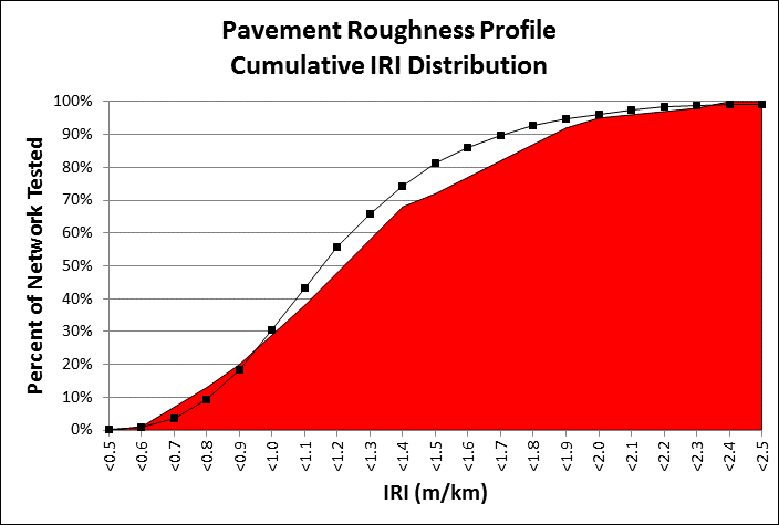
A highway concession may have thousands of 50 m sections. The percent of 50 m sections in each “bin” of IRI range from 0.5 to 2.5 m/km. For example, the figure shows that 50 percent of the sections must have an IRI of less than 1.25 m/km. The curve in the figure shows that about 60 percent of the sections have an IRI of less than 1.25 m/km which is compliant, but the curve moves into the red (non-compliant zone) for number of sections requiring an IRI of less than 0.9 m/km.
OBJECTIVES
A unique component of some of the concession agreements is the use of key performance indicator distributions such as those shown in figure above. These distributions add a new level of complexity to the prediction and budgeting of rehabilitation activities.
Typical PMS software applications allow for a large variety of goals during the forecasting analysis. However, they are not designed to meet the dynamic needs of the distribution analysis. This has proven to be one of the more difficult aspects of performing long term forecasting (ie. 5 years). The most optimal plan for a concessionaire is to plan rehabilitation activities such that in conjunction with the deterioration of non-rehabilitated sections just meets the distribution of IRI in the following year. Traditional pavement performace models for IRI would be developed through an age versus IRI graph. The following figure shows the age versus IRI graph for a typcial highway conditions with more than 5,000 pavement management sections each 50 m in length.
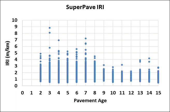
Clearly, it is not possible to fit a traditional performance curve thought this IRI data. Ideally, the overall roadway condition should be hovering just over the distribution line. In order to change the distribution, it is important to understand that improving the condition of an individual section will alter the shape of the distribution of all section with better performance. The means that many minor preventative maintenance activities on the network, although the most cost-effective treatment for the pavement, will not significantly change the distribution. By locating the poor performing sections on the distributions and simulating the results of the repair, an estimate of distribution can be created to assess any other areas of the curve that many need to be adjusted. For areas that affect the performance at around the 50 percent mark of the distribution, localized cost-effective rehabilitation and maintenance alternatives can be used to change the shape and ensure overall compliance.
The nature of the requirements for IRI, is such that pavement sections exhibiting an IRI of greater than 2.5 mm/m are scheduled for rehabilitation each year. The rehabilitation action taken may be very localized to address a bump or settlement and as long as the IRI for the 50 m section is reduced to below 2.5 m/km, the section is in compliance with the project requirements. Predicting when an individual section may exceed the 2.5 mm/m limit is very difficult as “rough” pavement sections may appear very quickly.
In order to develop an indication of the impact of the pavement maintenance and rehabilitation program on the distribution of IRI as compared to the concession IRI requirements, an analysis of the rate of change of IRI was completed. The average rate of change of IRI of 1.6 percent through the past 5 years was selected to represent the typical reduction in smoothness for sections that were not improved by maintenance or rehabilitation action. This average reduction in IRI was then applied to the all of the measured IRI for all 50 m sections that were not improved to determine the expected IRI for each section. For sections that were improved, the IRI values were “reset” and assigned to bins as shown in the following table. The bins are necessary because the result of maintenance to improve IRI will not result in the same IRI for all sections.
TABLE 2.2.10.1: IRI distribution
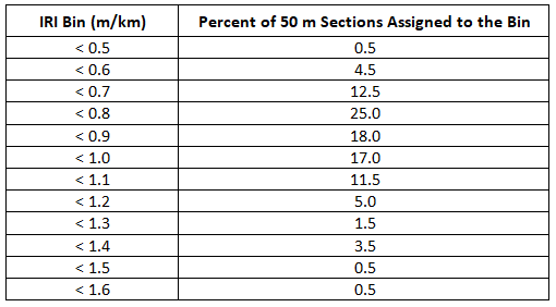
The percent of “improved” sections in each bin represents the expected improvement due to the rehabilitation action taken for pavement sections that exceeded an IRI value of 2.5 mm/m, i.e. 25 percent of sections were improved from an IRI of greater than 2.5 mm/m to less than 0.8 mm/m of roughness. The number of “improved” sections in each bin were then added back to the “deteriorated” IRI dataset based on the average deterioration of 1.6 percent per year to determine the new IRI cumulative distribution curve. The curve for 2018 is shown below.
A similar exercise was then completed for the next 5 years of the concession based on the maintenance and rehabilitation activities planned in the current 5-year plan and average annual rate of deterioration expected.
The cumulative distribution performance modeling described above permits the concessionaire to actively determine the impact of the current 5-year maintenance and rehabilitation plan on the cumulative distribution of IRI and to optimize their annual investments.
Paterson, W.D.O. International Roughness Index: Relationship to Other Measures of Roughness and Riding Quality. In Transportation Research Record 1084, National Research Councel, Washington, D.C., 1987.
Taylor, G.W., and J.D. Patton. Effects of Pavement Structure on Vehicle Fuel Consumption – Phase III Report CSTT-HVC-TR-068. National Research Council of Canada, 2006.
New Brunswick Department of Transportation (NBDOT). OMR – Asset Management Requirements Trans Canada Highway Project Attachment 61. Fredericton, New Brunswick, 1998.
Investment decisions for assets may also be allocated based on risk. For example, funding may be allocated to assets required to access remote communities. If the asset is compromised, residents may not be able to obtain access to essential services.The following chapters give an overview how different risks can be incorporated into asset management. The first chapter includes also an overview about the definition of risk in the context of asset management. The paragraphs aim at a better understanding of risk and how the different risks can be managed.
Different industries use many different definitions of risk and risk management (PIARC 2010). Some industries define risks narrowly and equate them to hazards or threats. This usage reflects the common, everyday definition of risks as threats or dangers. Others, however, increasingly use a much broader definition of risk. Many consider risks to include both possible threats and possible opportunities. The International Organization for Standardization (ISO) defines risk as “the effect of uncertainty on objectives,” (ISO 31000, 2009) and it notes that uncertainty could be positive or negative. Other definitions equate risk to variability or to the chance that desired outcomes won’t be achieved. The New Zealand Transport Agency, an international leader in risk and asset management, defines risk as “the chance of something happening that will have an impact on objectives. It is measured in terms of a combination of the likelihood of an event and its consequence.”
This expansive application of risk is evident in the definition of risk management used by the New South Wales (Australia) Government Asset Management Committee. It defines risk management as a systematic process to identify risks that may impact the organization’s objectives, analyze their consequences, and develop ongoing measures to treat them. These broader definitions of risk expand risk management to an enterprise-wide framework for setting priorities, assigning resources, and ensuring organizational success.
The broader definitions of risk emphasize that risks are not always negative. If risks are equated with uncertainty or variability, these definitions hold promise that risk could be positive as well as negative. PIARC has indicated that risk management could be called “opportunity management.” The field of financial management has long understood this implication. “No risk, no reward” is a basic investment premise. A financial advisor who only offers clients no-risk investments is unlikely to earn them a substantial return. Therefore, risk management is more than barricading an organization against all threats. Modern risk management involves protecting against excessive risk while capitalizing on opportunities that have acceptable risk levels. The English road organization notes that its risk management obligation is twofold. It must protect the public from hazards and threats to desired transportation outcomes, but it must also ensure that it identifies, evaluates, and capitalizes upon all reasonable opportunities.
Establishing the Context—this involves understanding and documenting the social, cultural, legal, regulatory, economic, and natural environment to which the agency is sensitive. The context allows risk management to be tailored to the agency’s needs and circumstances. Included in this step is the development of the organization’s risk policy designed around the agency’s unique objectives. These objectives can include issues such as improving network reliability by reducing the need for frequent maintenance and repair or providing the lowest reasonable whole-life costs for assets. Also included in this step is the creation of the agency’s internal and external risk management communication process. This process allows information to flow up and down through the agency and externally with key stakeholders.
A key element that agencies must consider and seamlessly integrate into the asset management framework is risk management. Risk is defined as “the positive or negative effects of uncertainty or variability upon agency objectives.” (see ISO 31000, 2009) Road organizations have for decades applied risk management at the project level. Increasingly, road organizations are integrating risk management more formally into their asset management processes, including the development of their asset management plans. This includes addressing the following questions (PIARC 2010):
The use of risk management among transportation agencies largely is limited to managing risk at the project level (PIARC 2008, PIARC 2013), generally during construction. Risk management at the project level helps to identify threats and opportunities to a project’s cost, scope, and schedule. However, road organizations need to recognize the growing need for a better understanding of risk management at program and organizational levels.
Today, the leading international transportation, banking, and insurance organizations have explored the benefits of risk management at the program and enterprise level and use it as a tool to protect their investments (PIARC 2016). It is important for road transportation agency officials to consider incorporating risk management into the decision-making process for several reasons. First, officials have seen the benefits of risk management at the project level. Second, they have heard from their international colleagues that risk management can pay dividends when used at the broader program and enterprise levels, particularly when agencies do not have enough funding to address their priorities. Third, managing risk is an integral step in following a comprehensive asset management framework, as described in the International Infrastructure Management Manual (IIMM, 2015), AASHTO Transportation Asset Management Manual - A Focus on Implementation (AASHTO, 2011), the UK Roads Liaison Group’s Road Infrastructure Asset Management Guidance Document (UKRLG and HMEP, 2013), etc.
Critical assets are those that are essential for supporting the social and business needs of both the local and national economy. These assets will have a high consequence of failure, but not necessarily a high likelihood of failure. These assets should be identified separately and assessed in greater detail as part of the asset management planning process.
By identifying critical assets, authorities can target and refine investigative activities, maintenance plans, and financial plans at the most crucial areas. Such assets may include special and major structures, such as estuarial crossings. Critical asset considerations may also include access to assets owned by third parties, such as substations, where access is via a single track road but accessibility is critical.
Criticality can be assessed by applying broad assumptions about the implications of failure, for example, whether the non-availability of a major structure or tunnel would have a significant impact on the local or possibly the national economy or whether higher trafficked roads are assumed to have a larger consequence of failure than lower trafficked roads. Using this approach, simple criteria can be defined to assess the loss of service. For example, the loss of use of a road may
Depending on the criticality of the asset, the risk management approach may be at a network level, by ensuring that diversions are available and have minimal impact; at an individual asset level; or at a detailed component level, with extensive consideration of failure modes.
The most commonly understood risks affecting the road service relate to safety. However, there are a wide range of other risks, and their identification and evaluation is a crucial part of the asset management process. Risks may include the following:
Risk Identification—in this step, the agency formally identifies the risks that could affect its objectives. These can be external, such as price changes, legislative actions, economic changes, extreme weather and climatic events, seismic events, or malevolent acts. Risks also can be internal, such as operational failures, data failures, conflicting internal program objectives, or a lack of trained personnel for key tasks. All risks are generally recorded in a formal risk register.
Risk Analysis—this step evaluates the probability of risk with its consequence. The calculation can be qualitative and based upon expert judgment, it can be quantified simply in a 1 to 10 scale, or it can be subject to complex mathematical modeling. Most such analyses are relatively simple. Regardless of the method used, the intent of this step is to understand the risks and their magnitude.
Risk assessment involves a determination of the likelihood and consequence of an event. Risk assessment allows the identified risks to be analyzed in a systematic manner to highlight which risks are the most severe and which are unacceptably high. An authority can then determine its level of exposure to the risk and the actions necessary to minimize that risk. An example of an assessment of the likelihood and consequence of a risk through a qualitative matrix approach is illustrated below.
Overall, risk is normally described as follows:
Risk = Likelihood × Consequence
Likelihood is the chance of an event happening, for example, a failure (asset as well as organizational) or service reduction. It can be measured objectively, subjectively, qualitatively, or quantitatively. It can be described using general or mathematical terms, such as frequency or probability. Issues to be considered include the following:
The likelihood of physical failure of an asset is related to the current condition of the asset, hence the importance of a realistic and accurate condition assessment. The likelihood of natural and external events is determined less easily, but scientific studies are usually available. The likelihood of other events, such as poor work practices or planning issues, can be difficult to ascertain.
Risk management is the framework to define the necessary treatments for the reduction of the different types of risk.
Risk Treatment—this decision making step applies what can be called the “five Ts”. These are to treat, tolerate, terminate, transfer, or take advantage of the risk. Although the steps are described as being distinct and separate, most manuals note that they tend to overlap and blend into each other. The steps of risk management occur within the context of continuous communication and consultation and continuous monitoring and review. The communication flows up and down the organization and into and out of it with stakeholders. Similarly, the monitoring occurs within the agency as well as outside it from oversight bodies, legislators, the media, and the public.
Risk Management—road authorities are required to manage a variety of risks at strategic, tactical, and operational levels. The likelihood and consequences of these risks can be used to inform and support their approach to asset management and inform key decisions regarding the performance of, investment in, and implementation of works programs. Successful implementation of the asset management framework requires a comprehensive understanding and assessment of the risks and consequences involved. Understanding risk enables the asset management process to address the issues identified.
A basic example of the consideration of risk is related to extreme weather events. All else being equal, programmatic decisions regarding projects should include risk and vulnerability analysis as one of the factors to consider as part of the asset management framework. Another illustration could be the case of an agency that has a well-crafted pavement program. The program relies on sound inventory data, good forecasting, methodical preventive maintenance, timely reactive treatments, and a well-balanced mix of pavement preservation, rehabilitation, and replacement. The agency has forecasted its program for the next five years and is confident it has developed a sound short-term and long-term pavement program that will achieve its short- and long-term performance targets. However, the risk of volatile construction prices creates a major program risk. If prices rise, the agency’s purchasing power will decrease and it will not be able to afford all the treatments it needs. If prices fall, it faces new opportunities to increase investments or achieve a higher level of service. A balanced risk management program would hedge against rising prices by methodically trying lower cost treatment innovations while closely monitoring construction prices. The degree of risk or uncertainty caused by price volatility would be documented, reported to stakeholders, and tracked as a risk to the department’s pavement objectives.
Understanding and management of risk is fundamental to effective asset management and should figure strongly in training and development programs for asset managers.
AASHTO (2011): AASHTO Transportation Asset Management Manual—A Focus on Implementation. American Association of State Highway and Transportation Officials (AASHTO), 1st Edition, USA, 2011
ISO 31000 (2009): Risk management. ISO standard, 2009.
IIMM (2015): IIMM - International Infrastructure Maintenance Manual. IPWEA, Institute of public works Australasia, 5th Edition, Australia, 2015
PIARC 2008. Risk Analysis for Road Tunnels, Technical Committee 3.3 – Road Tunnel Operation, ISBN: 2-8460-202-4 (https://www.piarc.org/ressources/publications/4/5877,2008R02-WEB.pdf).
PIARC 2010. Towards Development of a Risk Management Approach, Committee on Risk Management for Roads (3.2), ISBN: 2-84060-230-X (https://www.piarc.org/en/order-library/6741-en-Towards%20development%20of%20a%20risk%20management%20approach.htm).
PIARC 2013. Risk Evaluation, Current Practices for Risk Evaluation for Road Tunnels, Technical Committee C.4 – Road Tunnel Operation, ISBN: 978-2-84060-290-3 (https://www.piarc.org/ressources/publications/7/19445,2012R23-EN.pdf).
PIARC 2016. Role of Risk-Assessment in Policy Development and Decision-Making, Technical Committee 1.5 – Risk Management, ISBN: 978-2-84060-388-7 (https://www.piarc.org/ressources/publications/8/25153,2016R09EN-Risk-Management.pdf).
United Kingdom Roads Liaison Group (UKRLG) and Roads Maintenance Efficiency Programme (HMEP) (2013): Road Infrastructure Asset Management Guidance Document. Department for Transport, London. Last accessed July 24, 2015 (http://www.ukroadsliaisongroup.org/en/utilities/document-summary.cfm?docid=5C49F48E-1CE0-477F-933ACBFA169AF8CB).
These practices have been tested in several instances and case studies are being prepared. They will be presented here when available. If you want to share a case study, please contact assetmanagementmanual@piarc.org.
Lifecycle planning enables the asset managers to assess their decisions from a future oriented and sustainable point of view. There are different methods and solutions how to plan future maintenance activities on different types of assets. Lifecycle planning can be seen as the state of the art for finding the most efficient and adequate maintenance solutions. Thus, it should be applied especially on those assets where a high deterioration affects the different stakeholders.
In the following chapters the method of lifecycle planning as a part of modern asset management are presented. These chapters focus on modelling, planning, investment, resource allocations and procedures for generating a holistic lifecycle plan.
The objectives of lifecycle planning can be summarized as follows (UKRLG and HMEP, 2013):
Lifecycle planning describes the approach to maintaining an asset from construction to disposal. It involves the prediction of future performance of an asset, or a group of assets, based on investment scenarios and maintenance strategies. The lifecycle plan is the documented output from this process (UKRLG and HMEP, 2013).
Lifecycle plans may be used to demonstrate how funding and/or performance requirements are achieved through appropriate maintenance strategies with the objective of minimizing expenditure while providing the required performance over a specified period of time (PIARC 2000).
Lifecycle planning can be applied to all road infrastructure assets and can adopt a range of basic approaches depending on the maturity of the organization and the skills and capabilities of its staff. However, its application may be more beneficial to those assets that have the greatest value, require considerable funding, and are high risk and/or seen as critical assets. In some cases, complex approaches may be applied, and in these circumstances, higher quality data and predictive modelling techniques will often be needed. Where minimal data are available, a more basic or a risk-based approach may be adopted, as discussed in section 2.3.
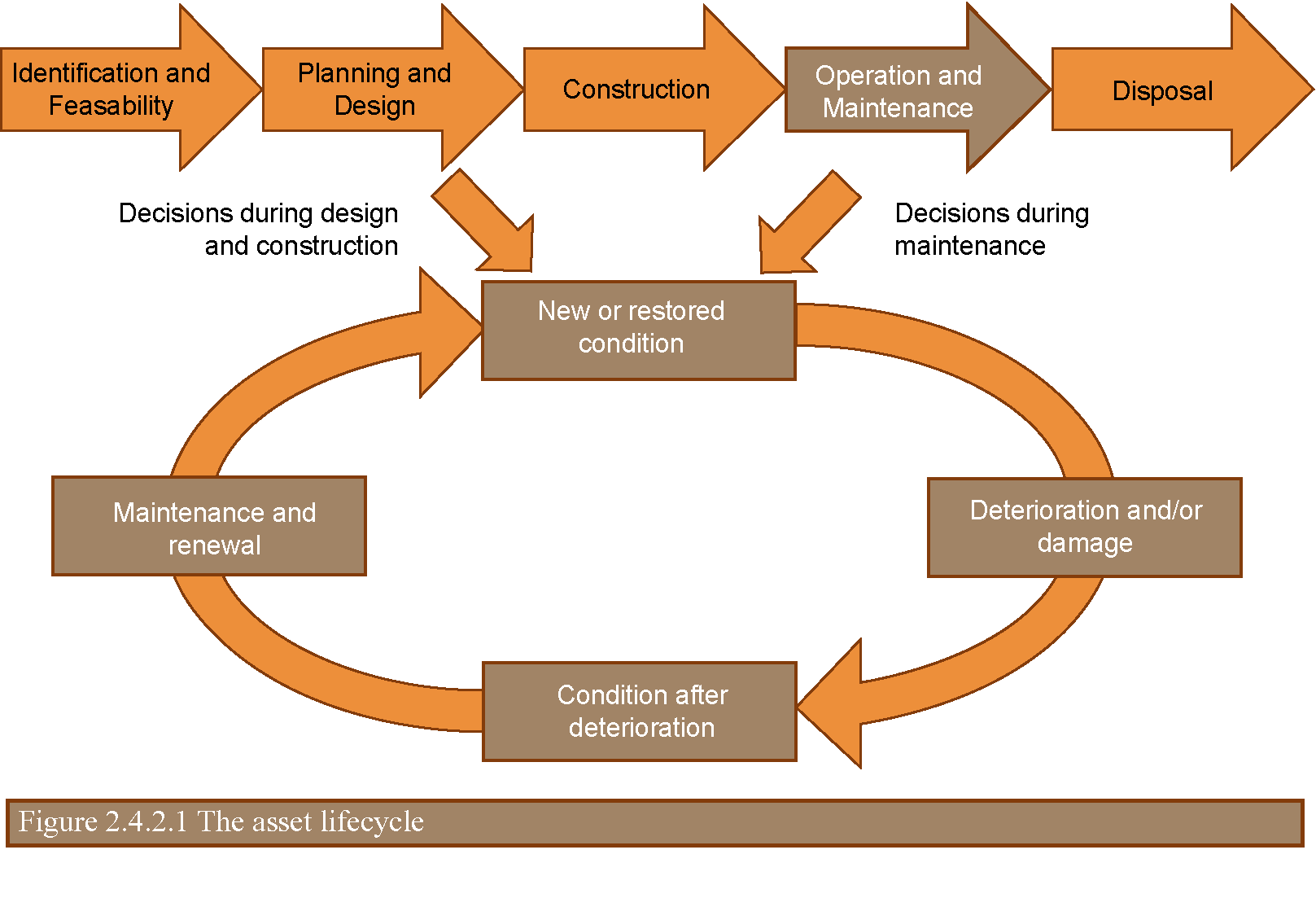
The lifecycle of an asset covers the following stages:
Maintenance strategies may be developed that consider different treatment options and balance renewal with routine maintenance. These strategies should take into consideration the service life for each treatment option and balance the costs over a planned period of time. The objective of this process is to provide a lifecycle plan for an asset that will support the implementation of the asset management strategy and objectives. When applying a lifecycle approach, the following questions may be answered for a short-, medium-, and long-term period of planning for each asset:
Adopting a lifecycle planning approach supports organizations in applying the principles of asset management to set maintenance standards that they can afford and/or that are desirable.
The desired performance is determined by setting the maintenance standards through developing performance targets, as described in section 1.4. Current asset performance is assessed through collecting information and data, based on the approach described in section 2.1, and monitoring performance, as described in section 2.2.
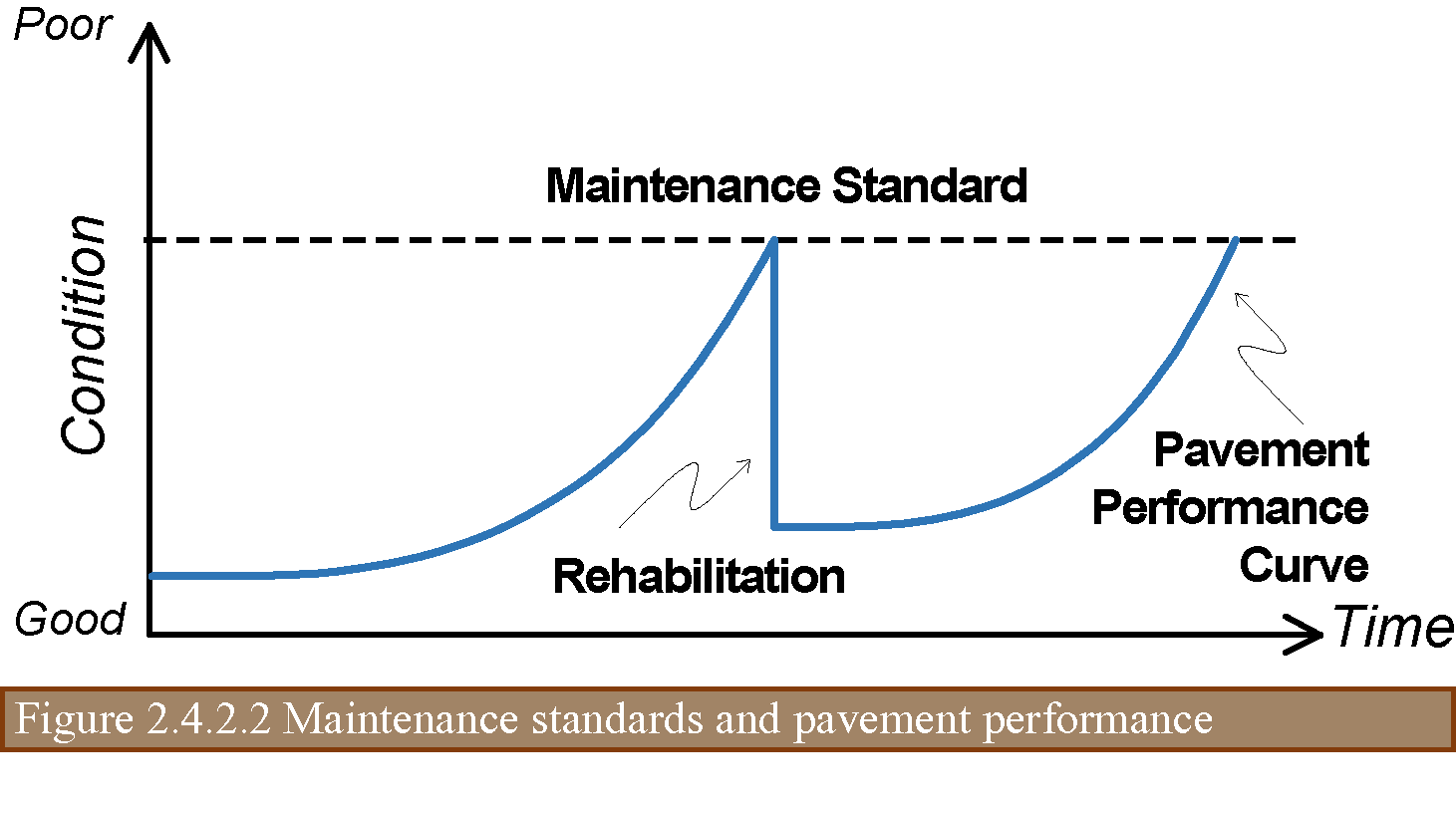
Typically, maintenance standards will have been selected for each asset type or group. These standards would normally represent the maintenance thresholds but may vary depending on the maturity of the organization that is applying lifecycle planning principles. It should be recognized that different performance requirements may also be adopted across different network hierarchies. For example, strategic roads may have different maintenance standards than less trafficked rural roads.
Where assets are to be maintained in a steady state, the lifecycle plan should be developed to meet existing performance requirements, as shown in Figure 2.4.2.2.
The approach to lifecycle planning adopted by an organization should be documented. Documentation should include the assumptions made, performance requirements, maintenance needs, the decision-making process, and the proposed maintenance strategy, including the timing of interventions.
A lifecycle planning approach will enable the maintenance strategy for all assets to be determined. However, the principal assets, where the greatest investment and/or risk will be incurred, should be considered as priorities when resources are scarce. Lifecycle planning is therefore likely to provide the greatest benefits for assets where large investments are made, including carriageways, footways, structures, and lighting.
The lifecycle planning process is shown in Figure 2.4.3.
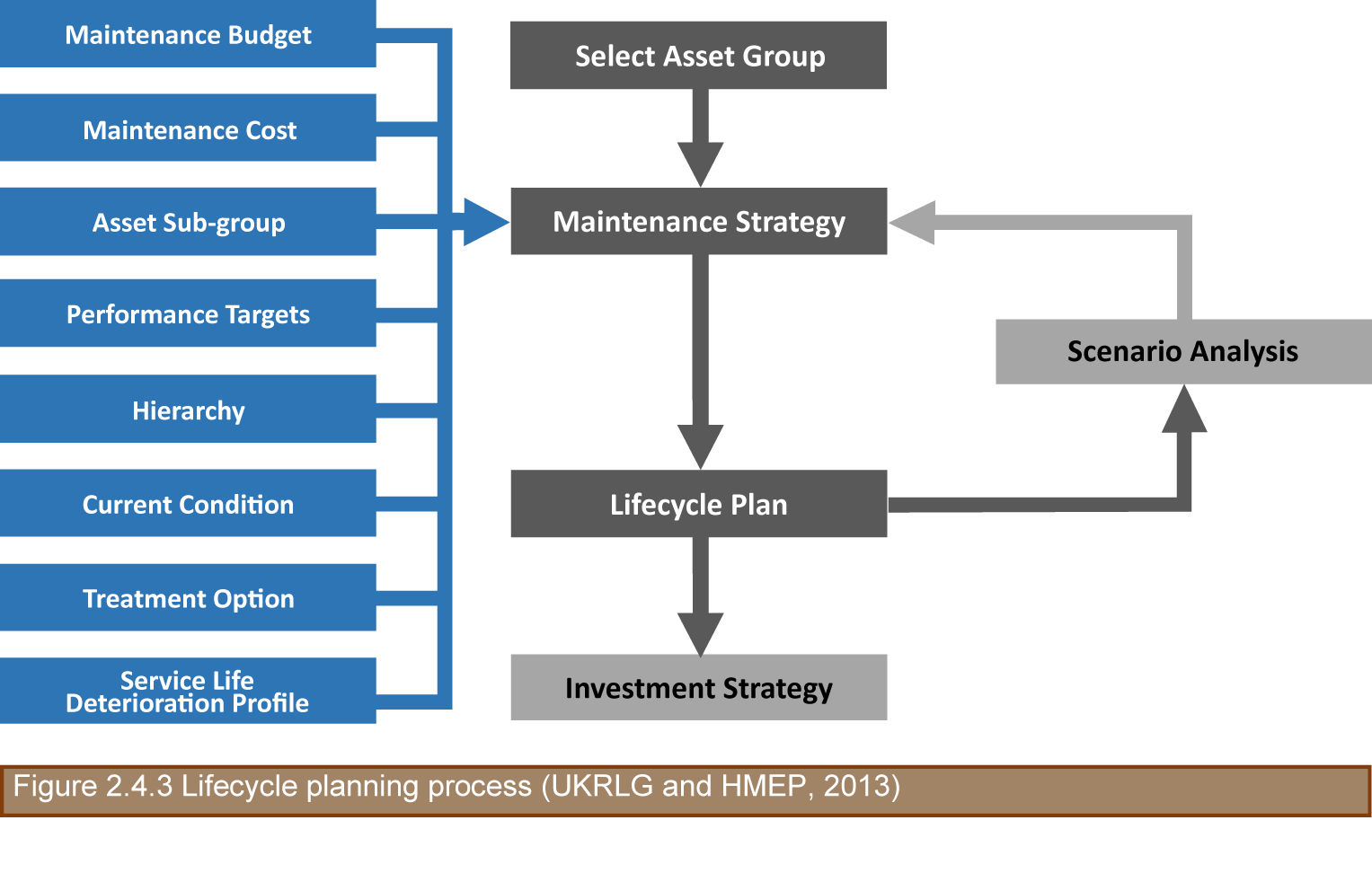
The degree to which each aspect is considered, as well as its sophistication, depends on the organization’s stage of maturity and the benefits it will achieve by investing in a lifecycle approach.
In developing a lifecycle plan, the asset group and/or its components should be identified at the network level, with similar assets grouped and aggregated together. The approach to selecting and grouping assets (see section 2.1) can be summarized as follows:
Asset data for lifecycle planning should be available from the organization via an asset management system, asset register, or maintenance management system (see section 4.1). Typically, the following is required to develop lifecycle plans:
The data requirements for lifecycle planning should be identified as part of the overall approach (see section 2.1). This may require specific data to be collected for relevant asset groups and their components.
The reliability, quality, and quantity of the data available, including inventory data and the historical performance of treatments, should be assessed before developing lifecycle plans. In general, the greater the confidence in the data available, the greater the confidence in the lifecycle plan.
Lifecycle plans should be updated regularly as new asset data becomes available. Plans should also be reviewed against any changes in the approach to asset management.
The inputs for lifecycle planning are as follows:
Asset inventory:This is the number, size, and/or dimensions of the asset that is to be analyzed. For a pavement maintenance project, this will be the length and width of the treatment area.
Analysis period: This is the duration over which the maintenance costs are to be evaluated. It should extend over at least one full lifecycle of the asset/treatment under consideration. Once an analysis period has been selected, it must be consistently applied across all maintenance options that are under consideration. Failure to do so will prevent meaningful comparisons between the lifecycle plans.
Treatment options: A treatment option needs to be selected for the lifecycle plan and can be prescribed for each maintenance strategy. Options could range from small-scale superficial works to wholesale replacement or reconstruction. A range of materials options or specification types should be considered. For a pavement maintenance project, treatment options will likely include a range of treatment depths.
Service life: The service life of an asset or treatment will determine the timing of future maintenance interventions. The use of realistic, achievable service lives is of primary importance in lifecycle planning. Service lives should be determined locally and be based on a number of factors, including performance history, material type, specification (including construction practices and workmanship), local environment, and demand (such as traffic levels and energy consumption, not necessarily applicable to all assets). These factors are based on practical experience, but they could be amended to suit local practices or performance histories.
Unit rates: This is the cost per unit measure (number/length/area/volume) to maintain an asset or part of an asset. It could, for example, be the price per square meter to apply a particular resurfacing treatment to a carriageway or the cost to replace a single lighting column. It is important that the engineer appreciates what is included in a particular rate and is aware of any assumptions that were used in deriving its value. This is considered to be essential to arrive at an accurate works cost.
Works costs: This is the direct cost of undertaking planned maintenance activities on site. Unit rates are used to estimate the works cost. The cost of site establishment, traffic management, and preliminaries should be included.
Routine maintenance costs: These are the (direct) ongoing costs of maintaining an asset in a safe and serviceable condition. These costs exclude cyclic activities such as sweeping and cleaning (because these are normally constant factors that will not vary according to treatment strategies or types). Routine maintenance costs need to be factored into the lifecycle plans if competing maintenance strategies are likely to result in significantly different ongoing costs.
Discount rates: Discounting is a technique used to compare costs (and benefits) that occur at different times throughout the analysis period. It works by adjusting these future costs (and benefits) to their present-day values. This practice enables competing maintenance options to be compared on a common basis, in that once a discount rate has been selected, it must be consistently applied across all maintenance options that are under consideration. Failure to do so will prevent meaningful comparisons between the whole-life costing results.
The outputs from the lifecycle process are as follows:
Investment strategy: The maintenance strategies, timing, and (direct and indirect) costs determined above will enable the production of a profile showing future investment in each year of the analysis period. By analyzing cost profiles across a program of works, it is possible to identify instances in the future where major works on several projects may coincide in a single year. These instances may pose future funding issues (and create network management and workload issues). Alternative maintenance strategies can then be considered to alleviate peak demands.
Discounted works cost: This is the present-day cost of all future maintenance requirements. It provides a basis for comparing alternative maintenance options and indicates the level of investment that will be required to meet future expenditure.
Once the need for maintenance has been identified, the input parameters above can be used to undertake a lifecycle analysis by considering the maintenance strategy to be adopted:
Do Nothing: Under this strategy, the organization would undertake reactive repairs for safety defects only. These repairs are likely to be superficial and would possibly be temporary in nature. The repairs would not arrest the decline of the asset, and frequent revisits are likely to be required. In the short term, routine maintenance costs are likely to be high due to the ongoing liability.
Do Minimum: Under this approach, the organization seeks to do the minimal amount of routine maintenance work to keep the asset safe and serviceable. Works will normally be restricted to the repair of safety defects; repairs will normally be permanent in nature, although they will add no value to the asset. In the context of a pavement project, this approach might be limited to the permanent repair of potholes only. These repairs would be undertaken on an isolated basis or may extend to small patches.
Do Something: This approach is likely to involve capital expenditure by an organization rather than routine expenditure. It may include the wholesale replacement or major repair of an asset to a level that will enhance its long-term durability and minimize future routine maintenance. A proactive approach may also be adopted, which means that repair takes place before the condition intervention level is reached. In the context of a pavement project, this approach could see the treatment of a section of pavement classified as being in need of maintenance.
It is recommended that more than one Do Something strategy is evaluated for each maintenance strategy in order to explore the range of available treatment types. For the Do Something strategies, the required timing of the initial maintenance intervention requires consideration. Options may include
If the latter (deferred) option is selected, then the additional routine maintenance costs need to be included in the lifecycle plan. In the context of a pavement project, the above factors could be realized. For example, a pavement nearing the end of its serviceable life may exhibit surface defects, such as potholes. If the initial treatment is deferred, then there will be an ongoing (possibly increasing) requirement to revisit the site during the period of deferment to carry out repairs to these defects. The costs of these repairs need to be included in the lifecycle plan. If the initial treatment is deferred, then more deterioration may occur to the pavement structure. This may result in a more extensive treatment eventually being required compared to the treatment that would otherwise have been implemented if the site were repaired earlier. By considering a range of treatment strategies and permutations on the type and timing of the initial intervention, an optimal maintenance strategy can be determined.
The maintenance strategy with the lowest net present value (NPV) is generally regarded as the most economically beneficial option (see Error: Reference source not found.4). However, whole-life costing is only one factor when selecting a preferred maintenance option. Other factors, such as engineering judgement, network operations, buildability, affordability, and risk management, also require consideration.
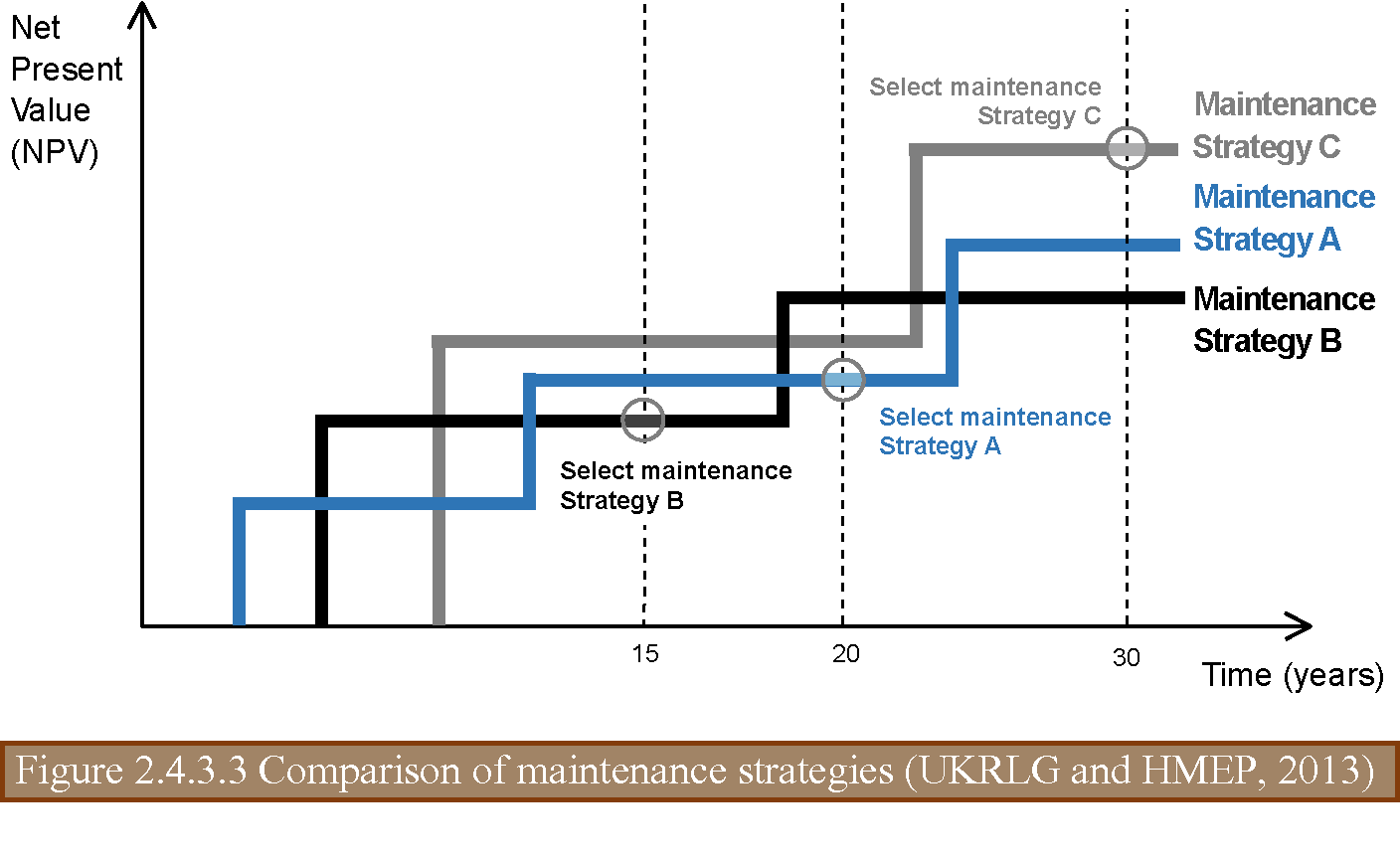
An organization may implement the above process according to its skills and capabilities, including data availability and performance models, as follows:
Where insufficient data are available, a more basic approach to lifecycle planning may be sufficient to meet the requirements of the organization. However, even standard approaches require data on asset hierarchy, inventory, and service life (estimated life of the treatment option). This approach may require assumptions to be made based on the experience and local/technical knowledge of the staff involved in the process. This experience and knowledge may include quantum as well as the current and predicted future performance of the asset. Any assumptions need to be documented and any significant risks set out.
A more advanced approach is likely to require higher quality data for performance or deterioration modelling in order to determine the service life of the proposed treatments (as described above). Subsequently, additional investment in data collection and asset management tools may be required in order to analyze and interrogate these data. Where this is the case, the argument should be made for any additional investment based on the benefits and efficiencies that can be obtained through adopting a more advanced approach.
The ability of an organization to develop performance models and model asset deterioration will support the advancement of its approach to lifecycle planning. These models have the capability to predict modes of deterioration and/or failure of the proposed treatment, as well as when the next intervention (the time for the asset to reach the end of its serviceable life) will occur. The approach can be advanced and highly complex approach or simple, depending on the capability of the organization. Two approaches to deterioration may be considered:
Service Life: This describes the life expectancy from construction to the next structural intervention based on industry best practice and local knowledge. This may vary according to traffic or environmental conditions. An organization’s own records of material performance should be a good reference.
Performance modelling: Deterioration profiles for an asset can be determined from a variety of sources, including historical performance, local knowledge, and best practice. Some organizations have developed bespoke deterioration profiles. These can be used for lifecycle planning with more sophisticated approaches to decision support. They will require a significant amount of data and potential calibration, which may be a complex and time consuming activity. These models may be part of the decision support component of the asset management tools (see section 4.1).
The decision-making process to select the investment strategy should align with the approach to asset management and, in particular, provide the most efficient and affordable way of achieving the performance requirements. Typically, the selection of maintenance strategies considers the following:
A number of techniques may be used to select the investment strategy, some of which are listed below. The International Infrastructure Maintenance Manual (IIMM, 2015) also gives advice on these decision-making techniques.
Risk-based evaluation focuses on minimizing the risk associated with the asset through an investment strategy while ensuring that any risks are managed at the minimum cost. The approach to risk management is described in section 2.3. Risk evaluation can be used as a decision-making technique on its own or considered with the other decision support techniques described below.
Whole-life cost is a cost-benefit analysis that quantifies the investment costs, including the cost of the treatment and subsequent maintenance interventions, against economic benefits, including safety, traffic delays, and pollution. These should be assessed for each maintenance strategy. The maintenance strategy with the lowest NPV over the period of analysis provides the lowest whole-life cost. Costs may be determined as described above. Benefits should be determined by each organization and considered in the context of its overall approach to asset management.
Multi-criteria analysis may be used to prioritize competing treatment options from which the maintenance strategy may be selected. A number of criteria may be selected that align with the levels of service and/or goals and objectives of the organization. Typically, these may include safety, serviceability, sustainability, and accessibility. A weighting to demonstrate the relative importance of these factors may be selected from which an overall score is determined. The necessity to meet statutory requirements needs to be reflected in the scoring. This technique can be used where benefits and costs are less tangible to define. However, it supports a qualitative assessment as well as a quantitative one.
The costs selected for any routine maintenance and asset renewal activities should be as reliable as possible. The selection of the maintenance strategy may be sensitive to the accuracy of this information.
A rigorous process should be developed for the collection and recording of cost data for the purposes of lifecycle planning. These cost data may be different from current contract rates because the data take other factors into account, such as overheads. Rates that are used should take into account inflation and be reviewed and updated as more cost information becomes available. The source of all cost data should be referenced.
The build-up of cost data is likely to include a number of assumptions, such as the inclusion of traffic management, contractor’s overheads, project design, and supervision costs. Such information may not be directly available from unit rates, which may be obtained from sources such as term maintenance contracts or framework contracts. Therefore, care needs to be taken in building up the rates in order to understand the item coverage.
The outcome of the lifecycle planning process is an investment strategy for the road infrastructure asset that comprises an asset group and its components and that is affordable and delivers the required performance at the minimum cost. In meeting this outcome, the investment strategy should also support the asset management strategy. A number of iterations, with different maintenance strategies, may be necessary to optimize the investment strategy.
In developing an investment strategy, the following issues should be considered:
What is the level of performance required to maintain a steady state condition and what is the budget required?
Lifecycle plans may be used to demonstrate the investment required to maintain the asset at its current level of performance. This is useful in cases where organizations are satisfied with the performance of their networks and to compare the impact of different funding scenarios.
What is the level of performance that can be achieved with a fixed budget?
Where an organization has fixed funding, lifecycle planning may be used to determine the performance of the asset for the funding allocated. It may also be used to target or prioritize funding in those areas that are most in need and to demonstrate the effect of reduced funding on the performance of assets over the short, medium, and long term.
What is the budget requirement to deliver the performance required?
Organizations can use lifecycle planning to determine future budget requirements. Performance targets may be selected for a hierarchy of asset groups and their components. In doing so, organizations may wish to consider the work needed to sustain the agreed performance requirements and any performance gaps.
What are the cross-asset considerations?
No organization will have unlimited funds to invest in an asset. Cross-asset prioritization, or “trade-off” techniques, may be used to determine where budgets are spent most effectively or at the lowest cost. Consideration of the risk, cost, and performance associated with each asset is key.
What is the timescale?
Lifecycle plans should be prepared for a period of at least 10 years.
Lifecycle plans are essential to assist senior decision makers in developing their financial plans and to substantiate any additional funding needed to achieve the required performance. Equally, they provide evidence of the effect on the asset if funding is not made available and the effect on the consequential future performance of the asset.
When organizations develop maintenance programs (e.g. lifecycle plans), they should ensure that their staff are appropriately trained and have the resources to build sustainable and realistic programs. Organizations should select adequate methods for asset management planning (e.g. lifecycle approach) appropriate to their maturity, needs, and resources.
The maturity levels for an organization undertaking lifecycle planning are shown in Table 2.4.9. Organizations may assess their maturity against this scale.
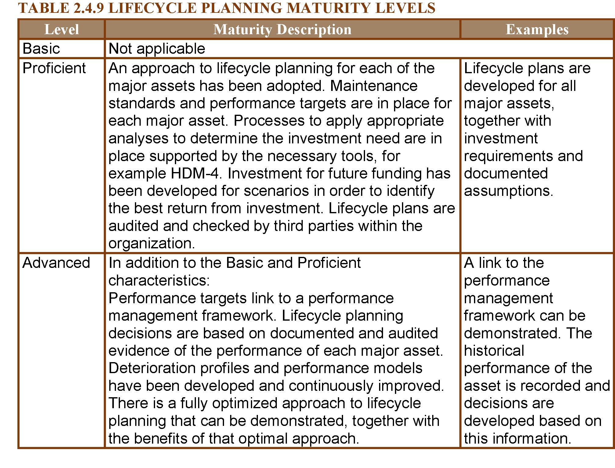
United Kingdom Roads Liaison Group (UKRLG) and Roads Maintenance Efficiency Programme (HMEP) (2013): Road Infrastructure Asset Management Guidance Document. Department for Transport, London. Last accessed July 24, 2015. http://www.ukroadsliaisongroup.org/en/utilities/document-summary.cfm?docid=5C49F48E-1CE0-477F-933ACBFA169AF8CB.
IIMM (2015): IIMM - International Infrastructure Maintenance Manual. IPWEA, Institute of public works Australasia, 5th Edition, Australia, 2015.
HDM-4 (2004): HDM-4 – The Highway Development and Management Series. World Road Association (PIARC/AIPCR), Paris, 2004.
PIARC 2000. Whole Life Costing of Roads – Flexible Pavements, Technical Committee 8 – Flexible Roads, ISBN: 2-94060-119-2 (https://www.piarc.org/ressources/publications/1/3762,08-09-e.pdf).
The following case studies are presented in this chapter:
Case study 1: HDM-4
Case study 2: Life-cycle analysis of Austrian pavements
The Roads Development and Management Tool (HDM-4) is a tool for the analysis, planning, management, and appraisal of road maintenance, improvements, and investment decisions. In 1998, PIARC was assigned the intellectual property s of HDM-4 on behalf of its original stakeholders (HDM-4, 2004). The HDM-4 analytical framework is based on the concept of pavement lifecycle analysis and is applied to predict the following over the lifecycle planning period of a road pavement (typically 15 to 40 years):
The model predicts road deterioration as a function of pavement construction characteristics, traffic loading, and climatic conditions and is directly affected by the standards of maintenance and improvements applied to repair the defects calculated. The long-term condition of the road pavement depends upon the application of these maintenance and improvement standards. Consequently, HDM-4 can determine the costs required to maintain the road to a standard defined by the user within HDM-4. The impacts of the road condition and road design standards on road users are quantified in terms of road user costs, which are made up of the following:
The socioeconomic effects comprise vehicle emissions, energy consumption, and other welfare benefits to the population served by the road network under analysis. HDM-4 is designed to make comparative cost estimates and economic analyses of different investment options or road maintenance strategies. The economic benefit from each road investment strategy is determined by comparing the total cost streams (transportation agency, road user, and socioeconomic costs) against a minimum standard, as illustrated in Figure 2.4.11.1.
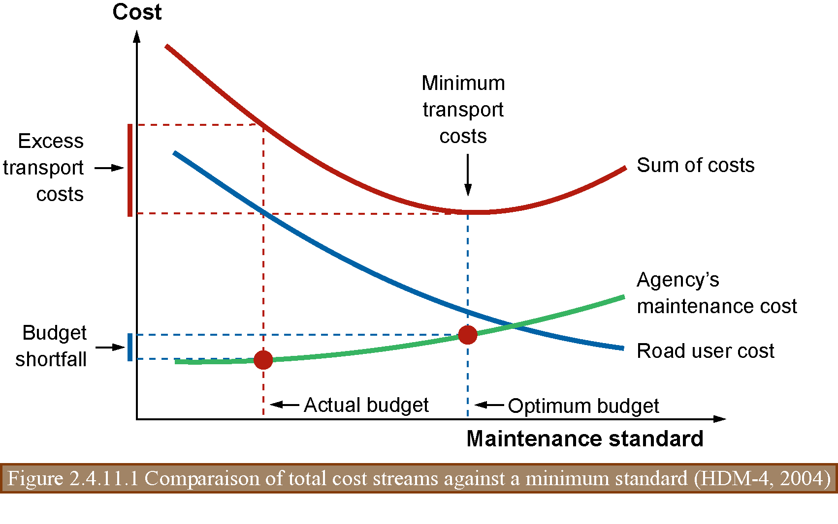
HDM-4 can be used in the lifecycle planning process by determining the benefits, costs, economic efficiency, and functional performance of the network by applying different maintenance and improvement standards to the network being analyzed. HDM-4 also allows organizations to determine the most economically efficient maintenance activities to carry out when budgets may not be sufficient to carry out all the work indicated.
ALFRED WENINGER-VYCUDIL, PMS-Consult – Deighton Europe, Austria
The Austrian Pavement Management System is used for a network-wide objective maintenance planning process in consideration of different aspects and demands on different decision levels (project-level, network-level, policy-level). At the moment, it is applied on the whole Federal road network (motorways and expressways) with a total length of more than 2,200 km as well as on the State road network in 7 of 9 Austrian states (Vorarlberg, Tyrol, Salzburg, Styria, Upper Austria, Lower Austria and Burgenland). Furthermore, a similar approach is being used to assess community road pavements and pavements on rural roads in 3 Austrian states.
The system employed for systematic pavement maintenance planning is based on life-cycle cost analysis (LCCA) that provides a framework for decision-making for maintenance measures in order to optimize efficiency in terms of the use of the resources available or in terms of pavement condition. The procedure employs cost-benefit analyses as well as a heuristic optimization process to identify the optimum maintenance treatment strategy in a given set of conditions.
OBJECTIVES
One of the key tasks throughout the decision-making process is the highlighting of needs for maintenance budget for the different assets. This output allows the road administration authorities to clearly show the policy makers the long-term development of the condition distribution of the pavement for different budgets or level of service and also the consequences of reductions in road maintenance funding. The results of the life-cycle analysis include:
The forecast of future condition using life-cycle analysis is the most efficient way to manage pavements and offers different opportunities for the road administration. The analysis enables the road administration to assess different options in managing their pavements. The assessment of different maintenance treatment strategies on a section level is a comprehensive basis for the definition of the short- to medium-term pavement construction programs. Long-term results allow budget, maintenance and rehabilitation planning and optimization. Phases with high investments can be detected on an early stage and specific investment programs can be prepared in advance.
Advanced systems like the Austrian PMS seek to assess the need for maintenance measures and maintenance funding over a specified period under study or observation on the basis of predictions of pavement performance. The Austrian PMS employs deterministic performance functions for the prediction of pavement performance. These models were derived directly from the data available in the context of different research projects funded by the ASFINAG (motorways and expressways) and the Federal Ministry of Transport, Innovation and Technology (BMVIT) for the state roads.
In the context of PMS analysis, different maintenance relevant data are included as follows:
Since, as a rule, each performance indicator (characteristic) represents only one aspect or one property of the road pavement, the individual dimensional values (technical parameters) obtained for the various characteristics first have to be standardized as dimensionless indices, then aggregated into sub-indices by applying weighting and combination rules, and finally aggregated into an overall index.
For transforming dimensional values, standardization functions (normalization) have been defined which enable an assessment of the damage or defect as a function of the importance of the road section (motorway, expressway, state road). The dimensionless values thus obtained, are aggregated by applying weighting and combination rules to yield a comfort and safety index (CSI) expressing riding safety and riding comfort and into a structural index (SI) which represents the structural capacity of the pavement. The total condition index (TCI) resulting from the sub-indexes can be usedfor calculating the benefit of a maintenance strategy as well as for defining the target function as part of the optimization process.
The result of an analysis is a proposal for an optimum maintenance treatment strategy for each road section analyzed (as a function of the conditions defined), which can be used for further evaluation at project level. By aggregating section-based results, one can also assess developments in terms of cost and pavement conditions across the entire network level and, finally, determine the optimum maintenance requirements. The following two figures show an example of the analysis, where Figure 2.4.11.2 represents a pavement condition distribution and Figure 2.4.11.3 shows the development of the maintenance backlog for different subnetworks in form of a comparison.
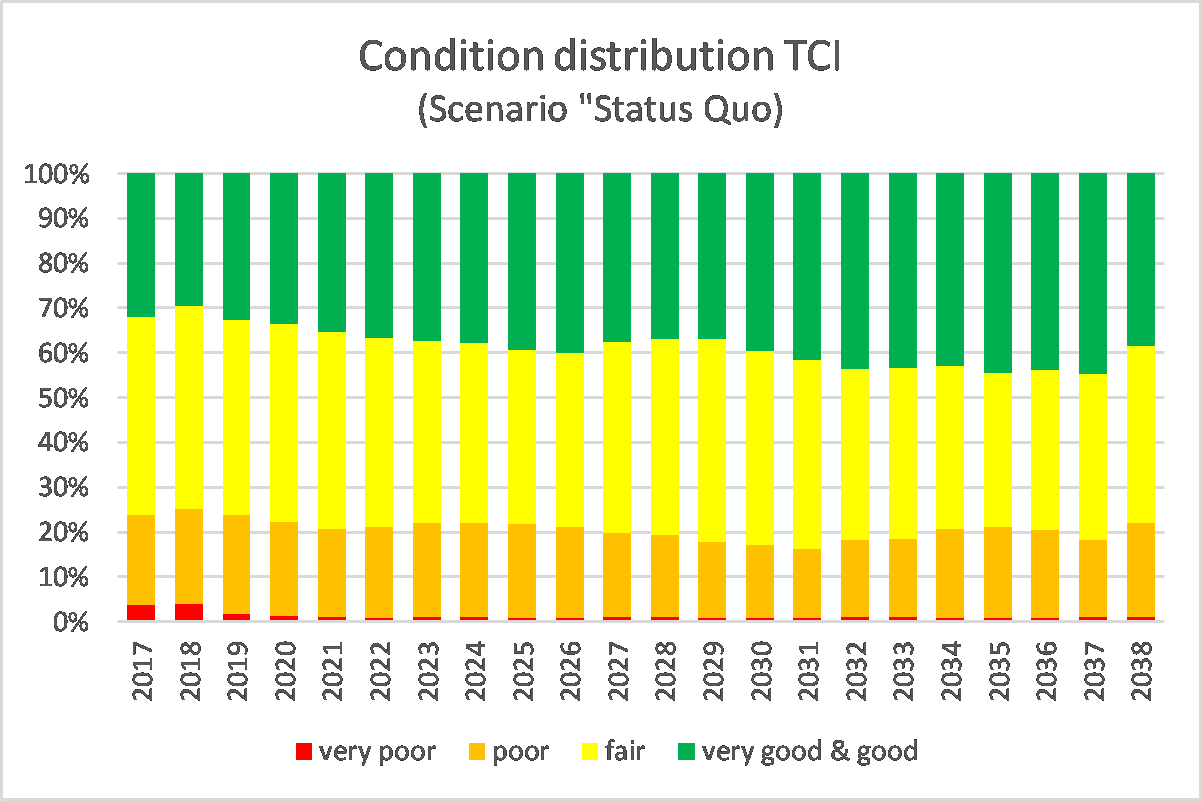
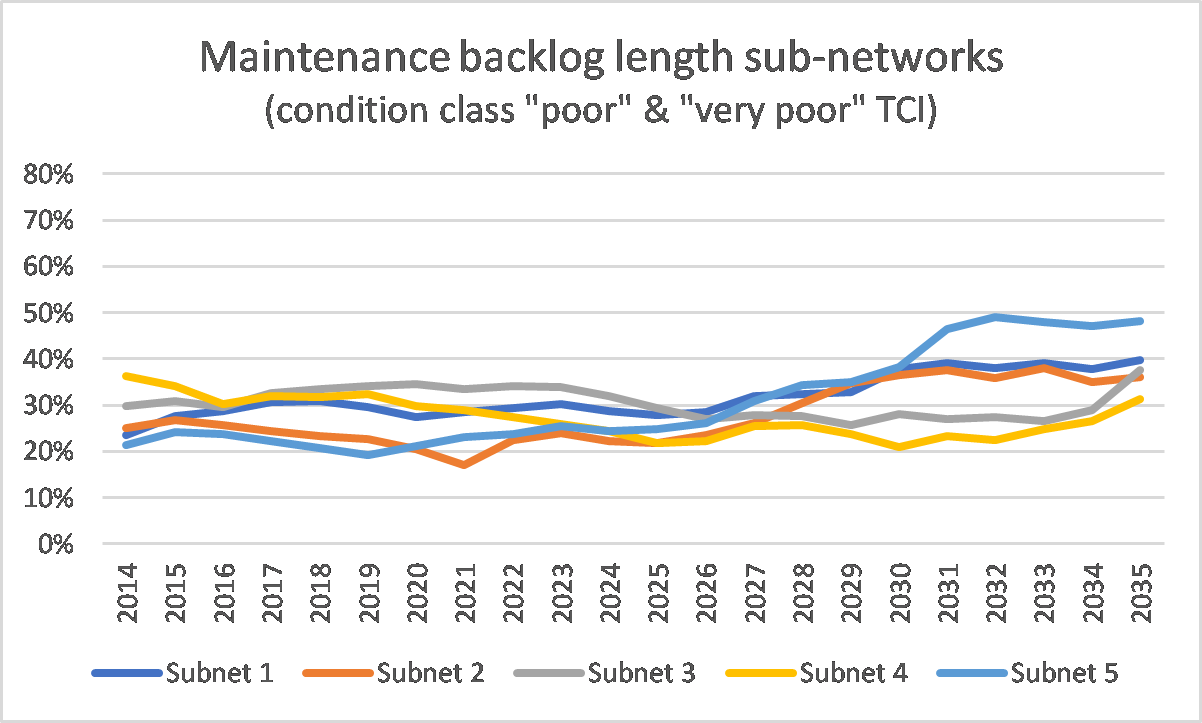
The practical application of the PMS relies on a computer-assisted asset management tool of Canadian origin (dTIMS© - Deighton Total Infrastructure Management System), which employs a deterministic optimization model for selecting the most effective maintenance treatment strategy in the context of life-cycle-cost analysis. In choosing the system, the decisive factor had been that algorithms and models can be modified and defined by the user as necessary to enable effective control or adaptation to the road network and general framework conditions.
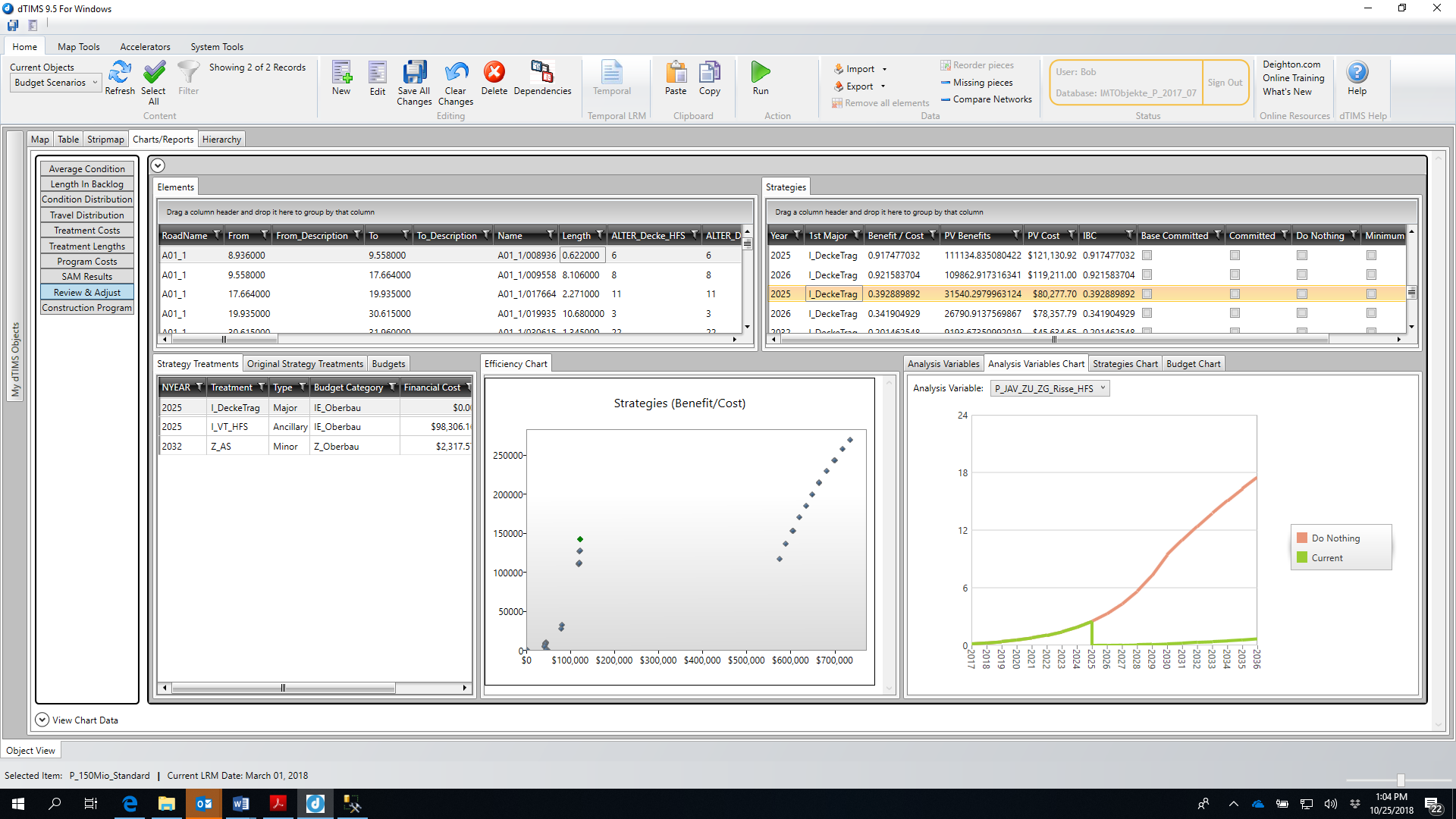
Pavement management systems using life-cycle cost analysis have become a standard in many countries around the world over the last 30 years. Beside having an objective instrument for underlining the need for maintenance investments, the solution enables the road administration to model future condition and investment needs for individual roadway segments and for the overall network. Austria is a good example how life-cycle cost analysis has and will be used as technical and strategic planning tool on the different road networks.
In recent years, many highway agencies have begun to focus on methods to address adverse events that cannot be tackled within the traditional risk-based approach. The focus of asset management activities is to begin from prevention against threats or events that may occur and that may degrade the performance of the asset itself to move towards a new comprehensive “Resilience-based” approach to be able to speed up recovery and restore asset functionality, once disruptive events have occurred. In the following sections, a brief definition of Resilience is provided, the difference between Risk and Resilience is highlighted and a general overview to facilitate the incorporation of Resilience into transportation assets and the corresponding strategies to improve resilience are presented.
The word “Resilience” comes from the field of structural mechanics and it refers to the ability of a material to withstand damaging actions after recovering from a previous yielding state. In the past 50 years, the derivative of this concept, in terms of “ability to recovery from adversities or disturbances”, has been extended to a wider range of fields, such as psychology, ecology, sociology, urban planning and so on. Within the Civil Engineering scope, since early 2000, resilience for transportation networks has been primarily made with reference to the response (impact and reactions) to natural hazards; however, it should be acknowledged that a resilience based approach should encompass all type of hazards (natural and man-derived ones). More recently, ISO introduced the concept of “Organizational Resilience” (ISO 2017) as “the ability of an organization to absorb and adapt in a changing environment to enable it to deliver its objectives” implying that Resilience in Road Asset Management may also deal with socio-organizational issues other than those coping with risk exposure to hazards.
Related to the context of Road Asset Management, it is worthy to highlight relevant differences between risk and resilience (see Fig. 1). While risk is a multi-faceted issue that can be associated with possible threats and opportunities, the risks themselves are not always negative (see the previous chapter) and that risk is strictly related to uncertainty affecting all the processes and interventions within asset management. On the other hand, resilience, although it is based on a risk evaluation, focus on issues related to the avoidance or minimization of disruption to the restoration of initial conditions and to maintain those latter or to the adaptation to a new operating scenario. Simplified, a resilience based approach also addresses the time, insofar as this will affect the recovery performance of the assets and the overall transportation system.
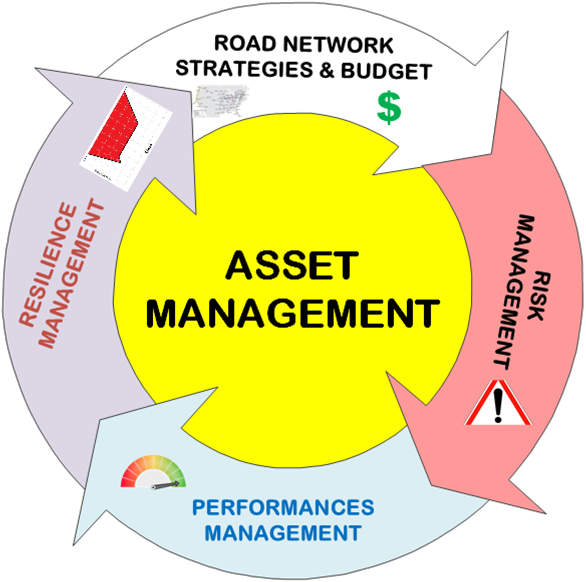
Figure 1. Resilience vs Risk and Asset management
Based on these premises, the risk evaluation framework is seamlessly integrated in the agency’s overall Asset Management approach. It also provides a sound starting point to develop resilience-based strategies and actions and to incorporate them in the overall decision-making process.
Following the identification of possible risks to asset functionality, a risk assessment process requires the definition and the likelihood and consequence of an event or scenario. In this manner, the choice of risk treatment, i.e. an intervention aimed at mitigating the likelihood and consequence of specific risk, shares the same common features with a resilience-based approach. Within a conventional risk-based approach, the likelihoods and consequences of different scenarios that may or may not include maintenance interventions are qualitatively or quantitatively evaluated in to provide information for prioritization and budget allocation. In a resilience-based approach however, these scenarios are enhanced by the time to recover in the aftermath of adverse events which can challenge the ability of the asset to effectively perform its desired function and to implement adaptation strategies.
For example, let us considers the need of improvement of the ability of a road network to withstands a seismic event (namely seismic vulnerability) with reference to its bridge stock (provided that it is possible to evaluate on a stochastic basis the damage scenario induced by a seismic excitation). By using a risk-based approach, a road manager would evaluate a prioritization of seismic retrofitting interventions within a restrained budget allocation. However, it is clear that it would be impossible to strengthen the entire bridge stock and therefore, following a severe earthquake, some bridges would likely be damaged yielding a network disruption that will take some time to recover. On the other hand, according to a resilience-based approach, several additional intervention strategies can be undertaken detailed as follows.
1) Bridges to be retrofitted may be carefully selected in order to reduce the impact of the overall traffic disruption induced by an earthquake and, according to this prioritization scheme, residual bridges that have not been retrofitted for budget constraints and that will suffer for major damages may be restored following the same aforementioned prioritization scheme in the ex-post period.
2) Retrofitting interventions can be adequately designed in order to speed-up repairing actions and therefore the recovery time.
Both strategies may contribute to an increase of the resilience of the road network insofar the functionality of road network will degrade to a lesser extent, as far as the performance level is concerned, because of the first strategy (see “A” section in figure 2). However, in this connection, it has to be acknowledged that a preventive retrofitting action shares the same approach of a risk-based methodology whereas a prioritization in the restoration phase will fall within a resilience-based process.
Furthermore, the network will be restored to its functional condition in a lesser time, according to the second strategy (see “B” and “C” sections in figure 2).
As far as the previous example is concerned, it appears clear that designing and implementing resilience-based strategies require a higher level of information on managed road networks as far as the local seismic characteristics, actual bridge stock structural condition and travel demand.
Keeping all these aforementioned points in mind, transportation organizations have been developing initiatives to incorporate the concept of resilience into transportation asset management systems for more than 10 years. To that end, the first requirement is to align understanding among engineers on what a resilient transportation infrastructure is (i.e. to establish a robust definition of resilience) and how to measure resilience.
The definition of resilience in transportation infrastructure systems have been discussed in the technical literature (Flannery et al., 2018; Zhou et al. 2019). The literature reveals that most definitions characterize resilience from one or both of the following two perspectives: the ability to maintain functionality under disruptions or deteriorating scenarios, and the time and resources required to restore the level of performance after disruptions. Resilience of transport system may be defined as ability of transport system to prepare for and adapt to major disruption, providing and maintaining an acceptable level of service or functionality and responding to and recovering rapidly from disruption. Following the past work of PIARC Technical Committee E.1 “Adaptation strategies and resiliency”, resilience is “an ability of a system or systems to survive and thrive in the face of a complex, uncertain and ever-changing future. Resilience approach is a way of thinking about both short-term cycles and long-term trends: minimizing traffic disruptions in the face of shocks and stresses, recovering rapidly when they do occur, and adapting steadily to become better and able to thrive as conditions continue to change. Within the context of critical infrastructure, the resilience process offers a cyclical, proactive and holistic extension of risk management practices”.
Therefore, resilience measurement includes time and the ability of the asset is able to perform at after an event occurs and before full functionality is recovered (see Figure 2). Resilience also includes adaptation, which implies recovering the infrastructure to a level above the original, which, again, implies strengthening the infrastructure to face a future with extreme events of greater magnitude, specifically those associated with climate change.
Furthermore, if multiple events of varying sizes are expected within a period of time there is the need to evaluate the maximization of the availability of the services provided by the system over time.
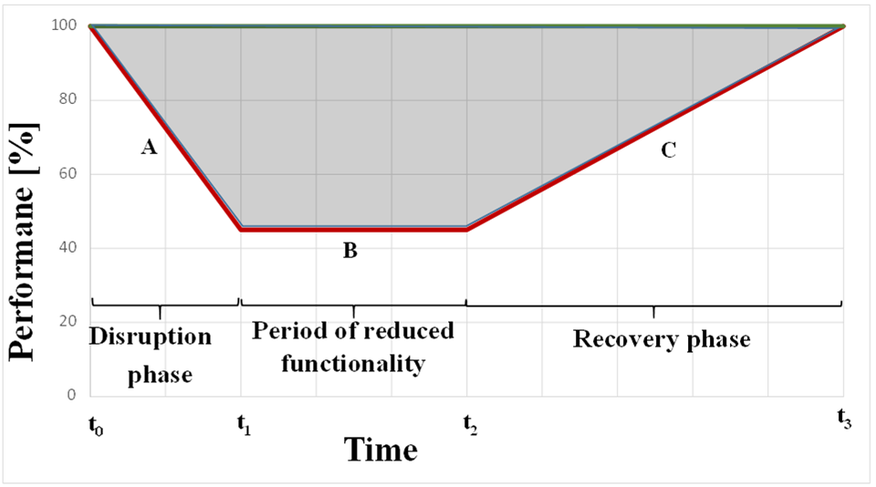
Figure 2. Conceptual phases characterizing resilience loss and corresponding measurement
The definition and illustration provided in Figure are consistent with the hypothesis formulated by some researchers that represent resilience as consisting of four contributing factors:
The level of robustness and redundancy are related to performance loss of the transportation system in disruption phase. Robustness measures the ability to withstand disaster-induced damage. Redundancy reflects the availability of alternative resources and at the system level refers to the existence of alternative roads that can provide the service in the event of a disruption or “system priorities that allow for alternative options, choices, and substitutions under stress” (Bruneau et al. 2003). Resourcefulness and Rapidity together determine the ability to restore functionality in the recovery phase.
In order to incorporate resilience into asset management processes, the transportation organization needs quantitative methods to measure resilience of their transport systems to threats that may cause failures. However, especially at an early stage of a resilience implementation process, it is suggested that qualitative measures should also be considered in addition to only a quantitative measure and analysis by using, for example, an Multi Criteria Analysis approach.
Generally, there are two steps to measure a resilience-related parameter. The first step is to assign a metric for measurement, and the second step is to establish evaluation criteria to assess the compliance with the metric. Currently, there is no overall measurement standard for resilience within the roadway network, both in terms of metrics and methods of assessment. Resilience metrics for transportation infrastructure used so far, can be divided into two categories: topological metrics and performance-based metrics (Nicolosi et al., 2022).
Metrics belonging to the first group use topological properties of transportation networks, such as shortest path length, average node degree or centrality (Aydin, 2018) and primarily focus on the layout of the transportation systems while ignoring the dynamic features and the operating condition. In other terms, topological properties such as, for example, the ratio between the number of links and number of nodes that is a numerical parameter related to the redundancy of network as far as the connectivity level is concerned, are mainly based on network layout.
The performance-based metrics measure systems’ resilience based on their performance over the period affected by disasters (disruption, period of reduced functionality and recovery according to Fig. 1). Three most widely used performance-based Measures of Resilience “MoR” identified in the literature are:
An example of a performance-based MoR of the type 1 is proposed in (Bruneau et al 2003 , Bocchini and Frangopol, 2010) and it is represented through Equation 1:
where: RL is defined as the resilience loss, Q(t) is the performance level of the system expressed in terms of percentage of the original asset condition value (prior to disruption event). The latter can be associated to a single or to an aggregate key performance indicator of the asset, or other functionality-based performance index such as the overall travelled time, the overall travelled distance or the overall generalized transport cost within the examined road network. It is worthy to note that the MoR parameter can be graphically defined as the shaded area shown in Figure 1.
For the second type of indicator, resilience is dynamically represented not merely as single parameter but rather as a time dependent function (as opposed to the other types of indicators, where resilience is a steady indicator) that represents the overall effects of disruption in the 3 phases following the occurrence of the event.
In the third type of MoR, resilience is defined as the expected ratio of demand satisfied by the network in the post-disaster phases with specific recovery costs. These indicators thus have two characteristics: 1) they explicitly consider transportation demand; and 2 ) they consider the dependence of the post-disruption phases on the economic resources committed.
Generally, the researchers consider the performance-based metrics more appropriate than topological metrics to measure the resilience of transportation systems, as the latter do not consider traffic flows in the network. However, it is worthy to highlight that some topological metrics have been suggested in order to evaluate redundancy properties of networks affecting overall resilience (Jovanović et al. 2018) and therefore such metrics may be justified in an early stage of a resilience implementation process within Road Asset Management. Among all the performance-based metrics, the third type MoR are preferable as they account for the performance of the system during the whole process, the real operating traffic condition s and the economic resources mobilized. Furthermore, the metrics that include economic resources required for recovery, which influence the recovery time, within the assessment of resilience, are more valuable than the others that usually consider recovery resources as constraints.
In the literature several approaches were proposed to measure the level of functionality of transportation systems and calculate performance based resilience metrics. These performance evaluation approaches were categorized as: optimization models, simulation models, probability theory models, fuzzy logic models, and data-driven models. Among all of them, optimization models are the most widely used.
The identification and implementation strategies to improve resilience in a transportation asset requires a comprehensive approach that is able to take into account all the possible and complex interdependencies between transportation system components and all the foreseeable hazards.
A simplified approach may start from the aforementioned resilience contributing factors (see section 2.5.2) according to which strategies can be grouped as or pro-active actions, if they are dealing with improving robustness and redundancy, and post event actions, if they are aiming at increasing resourcefulness and recovery speed.
In this connection, the former actions can be considered as mainly similar to the risk-reduction strategies (if any) that may have been already undertaken by management, whereas the latter ones can be regarded as peculiar for the resilience management.
ISO 22316 (2017) Organizational Resilience. ISO Standards , 2017.
Flannery, A., Pena, M. A., & Manns, J. (2018). Resilience in Transportation Planning, Engineering, Management, Policy, and Administration (No. Project 20-05; Topic 48-13).
Zhou, Y., Wang, J., & Yang, H. (2019). Resilience of transportation systems: concepts and comprehensive review. IEEE Transactions on Intelligent Transportation Systems, 20(12), 4262-4276.
Bruneau, M.; Chang, S. E.; Eguchi, R. T.; Lee, G. C.; O’Rourke, T. D.; Reinhorn, A. M.; Shinozuka, M.; Tierney, K.; Wallace, W. A. (2003). A Framework to Quantitatively Assess and Enhance the Seismic Resilience of Communities. Earthquake Spectra. 19 (4): 733–752. doi:10.1193/1.1623497.
P. Bocchini and D. M. Frangopol (2010). Optimal resilience- and cost-based postdisaster intervention prioritization for bridges along a highway segment, J. Bridge Eng., vol. 17, no. 1, pp. 117–129.
Nicolosi, V.; Augeri, M.; D’Apuzzo, M.; Evangelisti, A.; Santilli D.; (2022) A Probabilistic Approach to the Evaluation of Seismic Resilience in Road Asset Management, International Journal of Disaster and Risk Science, https://doi.org/10.1007/s13753-022-00395-5.
Aydin, N. Y., Duzgun, H. S., Wenzel, F., & Heinimann, H. R. (2018). Integration of stress testing with graph theory to assess the resilience of urban road networks under seismic hazards. Natural Hazards, 91(1), 37-68.
Jovanović A., Klimek P., Choudhary A., Schmid N., Linkov I., Øien K., Vollmer M., Sanne J.,
Andersson S. L., Székely Z., Molarius R., Knape T., Barzelay U., Nikolic M., Walther G., Lieberz D.,
Maraglino V. (2018) Analysis of existing assessment resilience approaches, indicators and data sources, Deliverable 2.1, SmartResilience Project: Indicators for Smart Critical Infrastructures.
These practices have been tested in several instances and case studies are being prepared. They will be presented here when available. If you want to share a case study, please contact assetmanagementmanual@piarc.org.